LOG#099. Group theory(XIX).

Posted: 2013/04/23 | Author: amarashiki | Filed under: Group Theory: basics, Physmatics | Tags: addition of angular momentum, angular momentum, angular momentum composition, Clebsch-Gordan coefficients, group theory, irreducible tensor operator, ITO, Quantum Mechanics, reduced matrix element, scalar operator, selection rules, vector operator, Wigner-Eckart theorem | Leave a comment

Final post of this series!

The topics are the composition of different angular momenta and something called irreducible tensor operators (ITO).

Imagine some system with two “components”, e.g., two non identical particles. The corresponding angular momentum operators are:

$J_1\cdot J_1, J_2\cdot J_2, J_1^z, J_2^z$

The following operators are defined for the whole composite system:

$J=J_1+J_2$

$J_z^T=J_z^1+J_z^2$

$J^2=(J_1+J_2)^2$

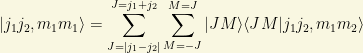
These operators are well enough to treat the addition of angular momentum: the sum of two angular momentum operators is always decomposable. A good complete set of vectors can be built with the so-called tensor product:

$\vert j_1j_2,m_1m_2\rangle =\vert j_1,m_1\rangle \otimes \vert j_2,m_2\rangle$

This basis $\vert j_1j_2,m_1m_2\rangle$ could NOT be an basis of eigenvectors for the total angular momentum operators $J^2_T,J_z^T$ . However, these vector ARE simultaneous eigenvectors for the operators:

$J_1\cdot J_1,J_2\cdot J_2,J_z^1, J_z^2$

The eigenvalues are, respectively,

$\hbar^2 j_1(j_1+1)$

$\hbar^2 j_2(j_2+1)$

$\hbar m_1$

$\hbar m_2$

Examples of compositions of angular momentum operators are:

i) An electron in the hydrogen atom. You have $J=l+s$ with $l=r\times p$ . In this case, the invariant hamiltonian under the rotation group for this system must satisfy

$\left[H,J\right]=0$

ii) N particles without spin. The angular momentum is $J=l_1+l_2+\cdots+l_N$

iii) Two particles with spin in 3D. The total angular momentum is the sum of the orbital part plus the spin part, as we have already seen:

$J=l+s=l_1+l_2+s_2+s_2$

iv) Two particles with spin in 0D! The total angular momentum is equal to the spin angular momentum, that is,

$J=S=s_1+s_2$

In fact, the operators $J^2,J_1\cdot J_1,J_2\cdot J_2,J_z$ commute to each other (they are said to be mutually compatible) and it shows that we can find a common set of eigenstates

$\vert j_1j_2,JM\rangle$

The eigenstates of $J^2, J_z$ , with eigenvalues $\hbar^2 J(J+1)$ and $\hbar M$ are denoted by

$\vert \Omega J,M\rangle$

and where $\Omega$ is an additional set of “quantum numbers”.

The space generated by $\vert \Omega,JM\rangle$ , for a fixed number $J$ , and $2J+1$ vectors, $-J\leq M\leq J$ , is an invariant subspace and it is also irreducible from the group theory viewpoint. That is, if we find a vector as a linear combination of eigenstates of a single particle, the remaining vectors can be built in the same way.

The vectors $\vert j_1j_1,JM\rangle$ can be written as a linear combination of those $\vert j_1j_1,m_1m_2\rangle$ . But the point is that, due to the fact that the first set of vectors are eigenstates of $J_1\cdot J_1,J_2\cdot J_2$ , then we can restrict the search for linear combinations in the vector space with dimension $(2j_1+1)(2j_2+1)$ formed by the vectors $\vert j,m\rangle$ with fixed $j_1,j_2$ quantum numbers. The next theorem is fundamental:

Theorem (Addition of angular momentum in Quantum Mechanics).

Define two angular momentum operators $J_1,J_2$ . Define the subspace, with $(2j_1+1)(2j_2+1)$ dimensions and $j_1\geq j_2$ , formed by the vectors

$\vert j_1j_2,m_1m_2\rangle=\vert j_1,m_1\rangle \otimes \vert j_2,m_2\rangle$

and where the (quantum) numbers $j_1,j_2$ are fixed, while the (quantum) numbers $m_1,m_2$ are “variable”. Let us also define the operators $J=J_1+J_2$ and $J^2,J_z$ with respective eigenvalues $J,M$ . Then:

(1) The only values that J can take in this subspace are

$J\in E=\left\{ \vert j_1-j_2\vert, \vert j_1-j_2+1\vert,\ldots,j_1+j_2-1,j_1+j_2\right\}$

(2) To every value of the number J corresponds one and only one set or series of $2J+1$ common eigenvectors to $J_z$ , and these eigenvector are denoted by $\vert JM\rangle$ .

Some examples:

i) Two spin 1/2 particles. $J=s_1+s_2$ . Then $j=0,1$ (in units of $\hbar=1$ ). Moreover, as a subspaces/total space:

$E(1/2)\otimes E(1/2)=E(0)\oplus E(1)$

ii) Orbital plus spin angular momentum of spin 1/2 particles. In this case, $j=l+s$ . As subspaces/total space decomposition we have

$E(l)\otimes E(1/2)=E(l+1/2)\oplus E(l-1/2)$ if $l\neq 0$

$E(l)\otimes E(1/2)=E(1/2)$ if $l=0$

iii) Orbital plus two spin parts. $j=l+s_1+s_2$ . Then, we have

$E(l)\otimes E(1/2)\otimes E(1/2)=E(l)\otimes (E(0)+E(1))=E(l)\otimes E(0)\oplus E(l)\otimes E(1)$

This last subspace sum is equal to $E(l)\oplus E(l+1)\oplus E(l)\oplus E(l-1)$ if $l\neq 0$ and it is equal to $E(0)\oplus E(1)$ if $l=0$ .

In the case we have to add several (more than two) angular momentum operators, we habe the following general rule…

$E=E(j_1)\otimes E(j_2)\otimes E(j_3)\otimes \ldots \otimes E(j_n)$

We should perform the composition or addition taking invariant subspaces two by two and using the previous theorem. However, the theory of the addition of angular momentum in the case of more than 2 terms is more complicated. In fact, the number of times that a particular subspace appears could not be ONE. A simple example is provided by 2 non identical particles (2 nucleons, a proton and a neutron), and in this case the total angular momentum with respect to the center of masses and the spin angular momentum add to form $j=l+s_1+s_2$ . Then

$E(l)\otimes E(1/2)\otimes E(1/2)=E(l)\otimes (E(0)\oplus E(1))=E(l)\otimes E(0)\oplus E(l)\otimes E(1)$

This subspace sum is equal to $E(l)\oplus E(l+1)\oplus E(l)\oplus E(l-1)$ if $l\neq 0$ and $E(0)\oplus E(1)$ if $l=0$ .

Clebsch-Gordan coefficients.

We have studied two different set of vectors and bases of eigentstates

(1) $\vert j_1j_2,m_1m_1\rangle$ , the common set of eigenstates to $J_1^2,J_2^2,J_{z1},J_{z2}$ .

(2) $\vert j_1j_1,JM\rangle$ , the common set of eigenstates to $J_1^2,J_2^2,J^2,J_z$ .

We can relate both sets! The procedure is conceptually (but not analytically, sometimes) simple:

$\displaystyle{\vert j_1j_2,JM\rangle=\sum_{m_1=-j_1}^{j_1}\sum_{m_2=-j_2;m_1+m_2=M}^{j_2}\vert j_1j_2,m_1m_2\rangle\langle j_1j_2,m_1m_2\vert JM\rangle}$

The coefficients:

$\boxed{\langle j_1j_2,m_1m_2\vert JM\rangle}$

are called Clebsch-Gordan coefficients. Moreover, we can also expand the above vectors as follows

$\displaystyle{\vert j_1j_2,m_1m_1\rangle=\sum_{J=\vert j_1-j_2\vert}^{J=j_1+j_2}\sum_{M=-J}^{M=J}\vert J M\rangle \langle J M\vert j_1j_2,m_1m_2\rangle}$

and here the coefficients

$\boxed{\langle J M\vert j_1j_2,m_1m_2\rangle}$

are the inverse Clebsch-Gordan coefficients.

The Clebsch-Gordan coefficients have some beautiful features:

(1) The relative phases are not determined due to the phases in $\vert j_1j_2,JM\rangle$ . They do depend on some coefficients $c_m$ . For any value of J, the phase is determined by recurrence! It shows that

$\langle j_1j_2,j_1 J-j_1\vert J,J\rangle \in \mathbb{R}^+$

This convention implies that the Clebsch-Gordan (CG) coefficients are real numbers and they form an orthogonal matrix!

(2) Selection rules. The CG coefficients $\langle j_1j_2,m_1m_2\vert J,M\rangle$ are necessarily null IF the following conditions are NOT satisfied:

i) $M=m_1+m_2$ .

ii) $\vert j_1-j_2\vert \leq J\leq j_1+j_2$

iii) $j_1+j_2+J\in \mathbb{Z}$

The conditions i) and ii) are trivial. The condition iii) can be obtained from a $2\pi$ rotation to the previous conditions. The two factors that arise are:

$R(2\pi)\vert j,m\rangle=(-1)^{2j}\vert j,m\rangle \leftrightarrow (-1)^{2J}=(-1)^{( j_1+j_2)}$

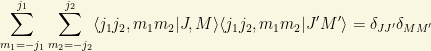
(3) Orthogonality.

$\displaystyle{\sum_{m_1=-j_1}^{j_1}\sum_{m_2=-j_2}^{j_2}\langle j_1j_2,m_1m_2\vert J,M\rangle\langle j_1j_2,m_1m_2\vert J' M'\rangle=\delta_{JJ'}\delta_{MM'}}$

$\displaystyle{\sum_{J=\vert j_1-j_2\vert}^{j_1+j_2}\sum_{M=-J}^{J}\langle j_1j_2,m_1m_2\vert J,M\rangle\langle j_1j_2,m'_1m'_2\vert J M\rangle=\delta_{m_1m'_1}\delta_{m_2m'_2}}$

(4) Minimal/Maximal CG coefficients.

In the case $J,M$ take their minimal/maximal values, the CG are equal to ONE. Check:

$\vert j_1j_2,J=j_1+j_2, J=M\rangle=\vert j_1j_2,m_1=j_1,m_2=j_2\rangle$

(5) Recurrence relations.

5A) First recurrence:

$C_J=\sqrt{J(J+1)-M(M-1)}\langle m_1m_2\vert J,M-1\rangle=$

$=\sqrt{j_1(j_1+1)-m_1(m_1+1)}\langle m_1+1,m_2\vert J,M\rangle+$

$+\sqrt{j_2(j_2+1)-m_2(m_2+1)}\langle m_1,m_2+1\vert J,M\rangle$

5B) Second recurrence:

$C'_J=\sqrt{J(J+1)-M(M+1)}\langle m_1,m_2\vert J,M+1\rangle=$

$=\sqrt{j_1(j_1+1)-m_1(m_1-1)}\langle m_1-1,m_2\vert J,M\rangle+$

$+\sqrt{j_2(j_2+1)-m_2(m_2-1)}\langle m_1,m_2-1\vert J,M\rangle$

These relations 5A) and 5B) are obtained if we apply the ladder operators $J_\pm$ in both sides of the equation defining the CG coefficients and using that

$J_\pm \vert JM\rangle=(J_{1\pm}+J_{2\pm})\vert JM\rangle$

$J_\pm \vert JM\rangle=\hbar \sqrt{J(J+1)-M(M\pm1)}\vert J,M\pm 1\rangle$

Irreducible tensor operators. Wigner-Eckart theorem.

There are 4 important previous definitions for this topic:

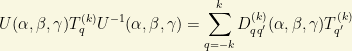
1st. Irreducible Tensor Operator (ITO).

We define $(2k+1)$ operators $T^{(k)}_q$ , with $q\in \left[-k,k\right]$ the standard components of an irreducible tensor operator (ITO) of order $k$ , $T^{(k)}$ , if these components transform according to the following rules

$\displaystyle{U(\alpha,\beta,\gamma)T^{(k)}_qU^{-1}(\alpha,\beta,\gamma)=\sum_{q=-k}^{k}D^{(k)}_{qq'}(\alpha,\beta,\gamma)T^{(k)}_{q'}}$

2nd. Irreducible Tensor Operator (II): commutators.

The $(2k+1)$ operators $T^{(k)}_q$ , $q\in \left[-k,k\right]$ , are the components of an irreducible tensor operator (ITO) of order k, $T^{(k)}$ , if these components satisfy the commutation rules

$\left[J_{\pm},T^{(k)}_q\right]=\hbar \sqrt{k(k+1)-q(q\pm 1)}T^{(k)}_{q\pm 1}$

$\left[ J_z,T^ {(k)}_q\right]=q\hbar T^{(k)}_q$

The 1st and the 2nd definitions are completely equivalent, since the 2nd is the “infinitesimal” version of the 1st. The proof is trivial, by expansion of the operators in series and identification of the involved terms.

3rd. Scalar Operator (SO).

We say that $S=T^0_0$ is an scalar operator, if it is an ITO with order k=0. Equivalently,

$U(\alpha,\beta,\gamma)SU^{-1}(\alpha,\beta,\gamma)=S$

One simple way to express this result is the obvious and natural statement that scalar operators are rotationally invariant!

4th. Vector Operator (VO).

We say that $V$ is a vector operator if

$\displaystyle{U(\alpha,\beta,\gamma)V^{(1)}_qU^{-1}(\alpha,\beta,\gamma)=\sum_{q=-1}^1D^{(1)}_{qq'}(\alpha,\beta,\gamma) V^{(1)}_{q'}}$

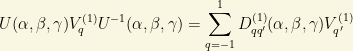
Equivalently, a vector operator is an ITO of order k=1.

The relation between the “standard components” (or “spherical”) and the “cartesian” (i.e.”rectangular”) components is defined by the equations:

$V_1=-\dfrac{1}{2}(V_x+iV_y)$

$V_0=V_z$

$V_{-1}=\dfrac{1}{2}(V_x-iV_y)$

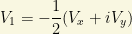
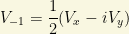
In particular, for the position operator $R=(r_1,r_0,r_{-1})$ , this yields

$r_1=-\dfrac{1}{\sqrt{2}}(x+iy)$

$r_=z$

$r_{-1}=\dfrac{1}{\sqrt{2}}(x-iy)$

Similarly, we can define the components for the momentum operator

$p=(p_1,p_0,p_{-1})$ or the angular momentum

$L=(L_+,L_-,L_z)\equiv (L_1,L_0,L_{-1})$

Now, two questions arise naturally:

1) Consider a set of $(2k+1)(2k'+1)$ operators, built from ITO $T^{(k)}_qT^{(k')}_{q'}$ . Are they ITO too? If not, can they be decomposed into ITO?

2) Consider a set of $(2k+1)(2J+1)$ vectors, built from certain ITO, and a given base of eigenvalues for the angular momentum. Are these vectors an invariant set? Are these vectors an irreducible invariant set? If not, can these vectors be decomposed into irreducible, invariant sets for certain angular momentum operators?

Some theorems help to answer these important questions:

Theorem 1. Consider $T^{(k_1)}_{q_1}, T^{(k_2)}_{q_2}$ , two irreducible tensor operators with $q_1\in \left[-k_1,k_1\right]$ and $q_2\in \left[-k_2,k_2\right]$ . Take $k$ and $q\in \left[-k,k\right]$ arbitrary. Define the quantity

$\displaystyle{S^{(k)}_q\equiv \sum_{q_1=-k_1}^{k_1}\sum_{q_2=-k_2}^{k_2}T^{(k_1)}_{q_1}T^{(k_2)}_{q_2}\langle k_1 k_2,q_1 q_2\vert k q\rangle}$

Then, the operators $S^{(k)}_q$ are the “standard” components of certain ITO with order $k$ . Moreover, we have, using the CG coefficientes:

$\displaystyle{T^{(k_1)}_{q_1}T^{(k_2)}_{q_2}=\sum_{q_1=-k}^{k}\sum_{q_2=\vert k_1-k_2\vert}^{k_1+k_2}S^{(k)}_q\langle k q\vert k_1 k_2, q_1 q_2\rangle}$

Theorem 2. Let $T^{(k)}_{q_1}$ be certain ITO and $\vert j_2 m_1\rangle$ a set of $(2j_2+1)$ eigenvectors of angular momentum. Let us define

$\displaystyle{\vert \omega_{JM }\rangle =\sum_{q_1=-k_1}^{k_1}\sum_{m_2=-j_2}^{j_2}\left(T^{(k_1)}_{q_1}\vert j_2 m_2\rangle\right)\langle k_1 j_2, q_1 m_2\vert J M\rangle}$

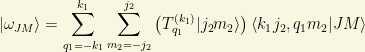
These vectors are eigenvectors of the TOTAL angular momentum:

$J^2\vert \omega_{JM}\rangle =J(J+1)\hbar^2\vert \omega_{JM}\rangle$

$J_z\vert \omega_{JM}\rangle=M\hbar \vert \omega_{JM}\rangle$

Note that, generally, these eigenstates are NOT normalized to the unit, but their moduli do not depend on $M$ . Moreover, using the CG coefficients, we algo get

$\displaystyle{T^{(k)}_{q_1}\vert j_2 m_2\rangle =\sum_{M=-J}^J\sum_{J=\vert k_1-j_2\vert}^{k_1+j_2}\vert J M\rangle \langle J M\vert k_1 j_2, q_1 m_2\rangle}$

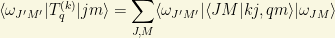
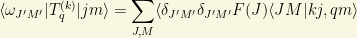
Theorem 3 (Wigner-Eckart theorem).

If $T^{(k)}_q$ is an ITO and some bases for angular momentum are provided with $\vert j_1 m_1\rangle$ and $\vert j_2 m_2\rangle$ , then

$\boxed{\langle j_2 m_2\vert T^{(k)}_{q}\vert j_1 m_1\rangle = \langle j_1 j_2, m_1 m_2\vert k q\rangle \dfrac{1}{2k+1}\langle j_2\vert \vert \mathbb{T}^{(k)}_q\vert\vert j_1\rangle}$

and where the quantity

$\boxed{\langle j_2\vert \vert \mathbb{T}^{(k)}_q\vert\vert j_1\rangle}$

is called the reduced matrix element. The proof of this theorem is based on (4) main steps:

1st. Use the $(2k+1)(2j+1)$ vectors (varying $q, m$ ), $T^{(k)}_q\vert j m\rangle$ .

2nd. Form the linear combination/superposition

$\displaystyle{\vert \omega_{JM}\rangle=\sum_{m,q}\left( T^{(k)}_q\vert j m\rangle\right)\langle k j, q m\vert J M\rangle}$

and use the theorem (2) above to obtain

$\langle J' M'\vert J M\rangle=\delta_{JJ}\delta_{MM}F(J)$

3rd. Use the CG coefficients and their properties to rewrite the vectors in the base with J and M. Then, irrespectively the form of the ITO, we obtain

$\displaystyle{T^{(k)}_q\vert j m\rangle=\sum_{J,M}\langle J M\vert k j, q m\rangle \vert \omega_{JM}\rangle}$

4th. Project onto some other different state, we get the desired result

$\displaystyle{\langle \omega_{J'M'}\vert T_q^{(k)}\vert j m\rangle=\sum_{J,M}\langle \omega_{J' M'}\vert \langle J M\vert k j, q m\rangle \vert \omega_{JM}\rangle}$

or equivalently

$\displaystyle{\langle \omega_{J'M'}\vert T_q^{(k)}\vert j m\rangle=\sum_{J,M}\langle \delta_{J' M'}\delta_{J'M'}F(J)\langle J M\vert k j,q m\rangle}$

i.e.,

$\displaystyle{\langle \omega_{J'M'}\vert T_q^{(k)}\vert j m\rangle=F(J)\langle J M\vert k j, q m\rangle}$

Q.E.D.

The Wigner-Eckart theorem allows us to determine the so-called selection rules. If you have certain ITO and two bases $\vert j_1,m_1\rangle$ and $\vert j_2, m_2\rangle$ , then we can easily prove from the Wigner-Eckart theorem that

(1) If $m_1-m_1\neq q$ , then $\langle j_1 m_1\vert T^{(k)}_q\vert j_2 m_2\rangle=0$ .

(2) If $\vert j_1-j_2\vert < k < j_1+j_2$ does NOT hold, then $\langle j_1 m_1\vert T^{(k)}_q\vert j_2 m_2\rangle=0$ .

These (selection) rules must be satisfied if some transitions are going to “occur”. There are some “superselection” rules in Quantum Mechanics, an important topic indeed, related to issues like this and symmetry, but this is not the thread where I am going to discuss it! So, stay tuned!

I wish you have enjoyed my basic lectures on group theory!!! Some day I will include more advanced topics, I promise, but you will have to wait with patience, a quality that every scientist should own! 🙂

See you in my next (special) blog post ( number 100!!!!!!!!).

LOG#098. Group theory(XVIII).

Posted: 2013/04/22 | Author: amarashiki | Filed under: Group Theory: basics, Physmatics | Tags: angular momentum, angular momentum algebra, angular momentum in QM, angular momentum operator, group theory, ladder operators, Pauli matrices, Quantum Mechanics, spin 1, spin 1/2, spin 2, spin 3/2, spin j, spin zero, SU(2) | Leave a comment

This and my next blog post are going to be the final posts in this group theory series. I will be covering some applications of group theory in Quantum Mechanics. More advanced applications of group theory, extra group theory stuff will be added in another series in the near future.

Angular momentum in Quantum Mechanics

Take a triplet of linear operators, $J=(J_x,J_y,J_z)$ . We say that these operators are angular momentum operators if they are “observable” or observable operators (i.e.,they are hermitian operators) and if they satisfy

$\boxed{\displaystyle{\left[J_i,J_j\right]=i\hbar\sum_k \varepsilon_{ijk}J_k}}$

that is

$\left[J_x,J_y\right]=i\hbar J_z$

$\left[J_y,J_z\right]=i\hbar J_x$

$\left[J_z,J_x\right]=i\hbar J_y$

The presence of an imaginary factor $i$ makes compatible hermiticity and commutators for angular momentum. Note that if we choose antihermitian generators, the imaginary unit is absorbed in the above commutators.

We can determine the full angular momentum spectrum and many useful relations with only the above commutators, and that is why those relations are very important. Some interesting properties of angular momentum can be listed here:

1) If $J_1,J_2$ are two angular momentum operators, and they sastisfy the above commutators, and if in addition to it, we also have that $\left[J_1,J_2\right]=0$ , then $J_3=J_1+J_2$ also satisfies the angular momentum commutators. That is, two independen angular momentum operators, if they commute to each other, imply that their sum also satisfy the angular momentum commutators.

2) In general, for any arbitrary and unitary vector $\vec{n}=(n_x,n_y,n_z)$ , we define the angular momentum in the direction of such a vector as

$J_{\vec{n}}=n\cdot J=n_xJ_x+n_yJ_y+n_zJ_z$

and for any 3 unitary and arbitrary vectos $\vec{u},\vec{v},\vec{w}$ such as $\vec{w}=\vec{u}\times\vec{v}$ , we have

$\left[J_{\vec{u}},J_{\vec{u}}\right]=i\hbar J_{\vec{w}}$

3) To every two vectors $\vec{a},\vec{b}$ we also have

$\left[\vec{a}\cdot\vec{J},\vec{b}\cdot\vec{J}\right]=i\hbar (\vec{a}\times \vec{b})\cdot \vec{J}$

4) We define the so-called “ladder operators” $J_+,J_-$ as follows. Take the angular momentum operator $J$ and write

$J_+=J_x+iJ_y$

$J_-=J_x-iJ_y$

These operators are NOT hermitian, i.e, ladder operators are non-hermitian operators and they satisfy

$J_+^+=J_-$

$J_-^+=J_+$

5) Ladder operators verify some interesting commutators:

$\left[J_x,J_+\right]=J_+$

$\left[J_x,J_-\right]=-J_-$

$\left[J_+,J_-\right]=2J_z$

6) Commutators for the square of the angular momentum operator $J^2=J_x^2+J_y^2+J_z^2$

$\left[J^2,J_k\right]=0,\forall k=x,y,z$

$\left[J^2,J_+\right]=\left[J^2,J_-\right]=0$

7) Additional useful relations are:

$J^2=\dfrac{1}{2}\left(J_+J_-+J_-J_+\right)+J_z^2$

$J_-J_+=J^2-J_z(J_z+I)$

$J_+J_-=J^2-J_z(J_z-I)$

8) Positivity: the operators $J_i^2,J_\pm,J_{+}J_{.},J_-J_+,J^2$ are indefinite positive operators. It means that all their respective eigenvalues are positive numbers or zero. The proof is very simple

$\langle \Psi \vert J_i^2\vert \Psi\rangle =\langle \Psi\vert J_iJ_i\vert\Psi\rangle =\langle \Psi\vert J^+_iJ_i\vert\Psi\rangle =\parallel J_i\vert\Psi\rangle\parallel\geq 0$

In fact this also implies the positivity of $J^2$ . For the remaining operators, it is trivial to derive that

$\langle \Psi\vert J_-J_+\vert\Psi\rangle\geq 0$

$\langle \Psi\vert J_+J_-\vert \Psi\rangle\geq 0$

since

$\langle\Psi\vert J_-J_+\vert\Psi\rangle =\langle\Psi\vert J_+^+J_+\vert\Psi\rangle=\parallel J_+\vert\Psi\rangle\parallel\geq 0$

$\langle\Psi\vert J_+J_-\vert\Psi\rangle =\langle\Psi\vert J_-^+J_-\vert\Psi\rangle =\parallel J_-\vert\Psi\rangle\parallel\geq 0$

The general spectrum of the operators $J^2, J_z$ can be calculated in a completely general way. We have to search for general eigenvalues

$J^2\vert\lambda,\mu\rangle=\lambda\vert\lambda,\mu\rangle$

$J_z\vert\lambda,\mu\rangle=\mu\vert\lambda,\mu\rangle$

The general procedure is carried out in several well-defined steps:

1st. Taking into account the positivity of the above operators $J^2,J_i^2,J_+J_-,J_-J_+$ , it means that there is some interesting options

A) $J^2$ is definite positive, i.e., $\lambda \geq 0$ . Then, we can write for all practical purposes

$\lambda=j(j+1)\hbar^2$ with $j\geq 0$

Specifically, we define how the operators $J^2$ and $J_z$ act onto the states, labeled by two parameters $j,m$ and $\vert j,m\rangle$ in the following way

$J^2\vert j,m\rangle =j(j+1)\hbar^2\vert j,m\rangle$

$J_z\vert j,m\rangle =m\hbar \vert j,m\rangle$

B) $J_+,J_-,J_+J_-$ are positive, and we also have

$J_-J_+\vert j,m\rangle =\left(J^2-J_z(J_z+I)\right)\vert j,m\rangle =(j-m)(j+m+1)\hbar^2\vert j,m\rangle$

$J_+,J_-\vert j,m\rangle =\left(J^2-J_z(J_z-I)\right)\vert j,m\rangle =(j+m)(j-m+1)\hbar^2\vert j,m\rangle$

That means that the following quantities are positive

$(j-m)(j+m+1)\geq 0 \leftrightarrow \begin{cases}j\geq m;\;\; j\geq -m-1\\ j\leq m;\;\; j\leq -m-1\end{cases}$

$(j+m)(j-m+1)\geq 0 \leftrightarrow \begin{cases}j\geq -m;\;\; j\geq m-1\\ j\leq -m;\;\; j\leq m-1\end{cases}$

Therefore, we have deduced that

(1) $\boxed{-j\leq m\leq j \leftrightarrow \vert m\vert \leq j}$ $\forall j,m$

(2) $\boxed{m=\pm j\leftrightarrow \parallel J_\pm \vert j,m\rangle \parallel^2=0}$

2nd. We realize that

(1) $J_+\vert j,m\rangle$ is an eigenstate of $J^2$ and eigenvalue $j(j+1)$ . Check:

$J^2\left(J_+\vert j,m\rangle \right)=J_+\left(J^2\vert j,m\rangle\right)=j(j+1)\hbar^2\left(J_+\vert j,m\rangle\right)$

(2) $J_+\vert j,m\rangle$ is an eigentstate of $J_z$ and eigenvalue $(m+1)$ . Check (using $\left[J_z,J_+\right]=J_+$ :

$J_z\left(J_+\vert j,m\rangle \right)=J_+(J_z+I)\vert j,m\rangle =(m+1)\hbar \left(J_+\vert j,m\rangle\right)$

(3) $J_-\vert j,m\rangle$ is an eigenstate of $J^2$ with eigenvalue $j(j+1)$ . Check:

$J^2\left(J_-\vert j,m\rangle \right)=J_-\left(J^2\vert j,m\rangle\right)=j(j+1)\hbar^2\left(J_-\vert j,m\rangle\right)$

(4) $J_-\vert j,m\rangle$ is an eigenvector of $J_z$ and $(m-1)$ is its eigenvalue. Check:

$J_z\left(J_-\vert j,m\rangle \right)=J_-(J_z-I)\vert j,m\rangle =(m-1)\hbar \left(J_-\vert j,m\rangle\right)$

Therefore, we have deduced the following conditions:

1) if $m\neq j$ , equivalently if $m\neq -j$ , then the eigenstates $J_+\vert j,m\rangle$ , equivalently $J_-\vert j,m\rangle$ , are the eigenstates of $J^2,J_z$ . The same situation happens if we have vectors $J_+^p\vert j,m\rangle$ or $J_-^q\vert j,m\rangle$ for any $p,q$ (positive integer numbers). Thus, the sucessive action of any of these two operators increases (decreases) the eigenvalue $m$ in one unit.

2) If $m=j$ or respectively if $m\neq -j$ , the vectors $J_+\vert j,m\rangle$ , respectively $J_-\vert j,m\rangle$ are null vectors:

$\exists p\in \mathbb{Z}/\left\{J_+^p\vert j,m\rangle\neq 0,J_+^{p+1}\vert j,m\rangle=0\right\}$ , $m+p=j$ .

$\exists q\in \mathbb{Z}/\left\{J_-^q\vert j,m\rangle\neq 0,J_-^{q+1}\vert j,m\rangle=0\right\}$ , $m-q=-j$ .

If we begin by certain number $m$ , we can build a series of eigenstates/eigenvectors and their respective eigenvalues

$m-1,m-2,\ldots,m-q=-j$

$m+1,m+2,\ldots,m+q=j$

So, then

$m+p= j$

$m-q=-j$

$2m=q-p$

$2j=p+q$

And thus, since $p,q\in\mathbb{Z}$ , then $j=k/2,k\in \mathbb{Z}$ . The number $j$ can be integer or half-integer. The eigenvalues $m$ have the same character but they can be only separated by one unit.

In summary:

(1) The only possible eigenvalues for $J^2$ are $j(j+1)$ with $j$ integer or half-integer.

(2) The only possible eigenvalues for $J_z$ are integer numbers or half-integer numbers, i.e.,

$\boxed{m=0,\pm \dfrac{1}{2},\pm 1,\pm\dfrac{3}{2},\pm 2,\ldots,\pm \infty}$

(3) If $\vert j,m\rangle$ is an eigenvector for $J^2$ and $J_z$ , then

$J^2\vert j,m\rangle=j(j+1)\hbar^2\vert j,m\rangle$ $j=0,1,2,\ldots,$

$J_z\vert j,m\rangle=m\hbar\vert j,m\rangle$ $-j\leq m\leq j$

We have seen that, given an state $\vert j,m\rangle$ , we can build a “complete set of eigenvectors” by sucessive application of ladder operators $J_\pm$ ! That is why ladder operators are so useful:

$J_+\vert j,m\rangle, J_+^2\vert j,m\rangle, \ldots, J_-\vert j,m\rangle, J_-^2\vert j,m\rangle,\ldots$

This list is a set of $(2j+1)$ eigenvectors, all of them with the same quantum number $j$ and different $m$ . The relative phase of $J^p_\pm\vert j,m\rangle$ is not determined. Writing

$J_\pm\vert j,m\rangle =c_m\vert j,m+1\rangle$

from the previous calculations we easily get that

$\parallel J_+\vert j,m\rangle\parallel^2=(j-m)(j+m+1) \hbar^2\langle j,m\vert j,m\rangle$

$\vert c_m\vert^2=(j-m)(j+m+1)\hbar^2=j(j+1)\hbar^2-m(m+1)\hbar^2$

$\parallel J_-\vert j,m\rangle \parallel^2=(j+m)(j-m+1)\hbar^2\langle j,m\vert j,m\rangle$

$\vert c_m\vert^2=(j+m)(j-m+1)\hbar^2=j(j+1)\hbar^2-m(m-1)\hbar^2$

The modulus of $c_m$ is determined but its phase IS not. Remember that a complex phase is arbitrary and we can choose it arbitrarily. The usual convention is to define $c_m$ real and positive, so

$J_+\vert j,m\rangle =\hbar \sqrt{j(j+1)-m(m+1)}\vert j,m+1\rangle$

$J_-\vert j,m\rangle =\hbar \sqrt{j(j+1)-m(m-1)}\vert j,m-1\rangle$

Invariant subspaces of angular momentum

If we addopt a concrete convention, the complete set of proper states/eigentates is:

$B=\left\{ \vert j,-j\rangle ,\vert j,-j+1\rangle,\ldots,\vert j,0\rangle,\ldots,\vert j,j-1\rangle,\vert j,j\rangle\right\}$

This set of eigenstates of angular momentum will be denoted by $E(j)$ , the proper invariant subspace of angular momentum operators $J^2,J_z$ , with corresponding eigenvalues $j(j+1)$ .

The previously studied (above) features tell us that this invariant subspace $E(j)$ is:

a) Invariant with respect to the application of $J^2,J_z$ , the operators $J_x,J_y$ , and every function of them.

b) $E(j)$ is an irreducible subspace in the sense we have studied in this thread: it has no invariant subspace itself!

The so-called matrix elements for angular momentum in these invariant subspaces can be obtained using the ladder opertors. We have

(1) $\langle j,m\vert J^2\vert j',m'\rangle = j(j+1)\hbar^2 \delta_{jj'}\delta_{mm'}$

(2) $\langle j,m \vert J_z\vert j',m'\rangle =m\hbar \delta_{jj'}\delta_{mm'}$

(3) $\langle j,m\vert J_+\vert j',m'\rangle =\hbar \sqrt{j(j+1)-m'(m'+1)}\delta_{jj'}\delta_{m,m'+1}$

(4) $\langle j,m\vert J_-\vert j',m'\rangle =\hbar \sqrt{j(j+1)-m'(m'-1)}\delta_{jj'}\delta_{m,m'-1}$

Example(I): Spin 0. (Scalar bosons)

If $E(0)=\mbox{Span}\left\{ \vert 0\rangle\right\}$

This case is trivial. There are no matrices for angular momentum. Well, there are…But they are $1\times 1$ and they are all equal to cero. We have

$J^2\vert 0\rangle =0\hbar^2=0(0+1)\hbar^2\cdot 1=0$

$J_x=J_y=J_z=J_+=J_-=0$

Example(II): Spin 1/2. (Spinor fields)

Now, we have $E(1/2)=\mbox{Span}\left\{\vert 1/2,-1/2\rangle,\vert 1/2,1/2\rangle\right\}$

The angular momentum operators are given by multiples of the so-called Pauli matrices. In fact,

$J^2=\dfrac{3}{4}\hbar^2\begin{pmatrix}1 & 0\\ 0 & 1\end{pmatrix}=\dfrac{3\hbar^2}{4}I=\dfrac{3\hbar^2}{4}\sigma_0$

$J_x=\dfrac{\hbar}{2}\begin{pmatrix} 0 & 1\\ 1 & 0\end{pmatrix}=\dfrac{\hbar}{2}\sigma_x$

$J_y=\dfrac{\hbar}{2}\begin{pmatrix} 0 & -i\\ i & 0\end{pmatrix}=\dfrac{\hbar}{2}\sigma_y$

$J_z=\dfrac{\hbar}{2}\begin{pmatrix} 1 & 0\\ 0 & -1\end{pmatrix}=\dfrac{\hbar}{2}\sigma_z$

and then $J_k=\dfrac{\hbar}{2}S_k=\dfrac{\hbar}{2}\sigma_k$ and $J^2=\dfrac{3}{4}\hbar^2I=\dfrac{3}{4}\hbar^2 \sigma_0$ .

The Pauli matrices have some beautiful properties, like

i) $\sigma_x^2=\sigma_y^2=\sigma_z^2=1$ The eigenvalues of these matrices are $\pm 1$ .

ii) $\sigma_x\sigma_y=i\sigma_x$ , $\sigma_y\sigma_z=i\sigma_x$ , $\sigma_z\sigma_x=i\sigma_y$ . This property is related to the fact that the Pauli matrices anticommute.

iii) $\sigma_j\sigma_k=i\varepsilon_{jkl}\sigma_l+\delta_{jk}I$

iv) With the “unit” vector $\vec{n}=\left(\sin\theta\cos\psi,\sin\theta\sin\psi,\cos\theta\right)$ , we get

$\vec{n}\cdot \vec{S}=\begin{pmatrix} \cos\theta & e^{-i\psi}\sin\theta\\ e^{i\psi}\sin\theta & -\cos\theta\end{pmatrix}$

This matrix has only two eigenvalues $\pm 1$ for every value of the parameters $\theta,\psi$ . In fact the matrix $\sigma_z+i\sigma_x$ has only an eigenvalue equal to zero, twice, and its eigenvector is:

$e_1=\dfrac{1}{\sqrt{2}}\begin{pmatrix} -i\\ 1\end{pmatrix}$

And $\sigma_z-i\sigma_x$ has only an eigenvalue equal to zero twice and eigenvector

$e_2=\dfrac{1}{\sqrt{2}}\begin{pmatrix} i\\ 1\end{pmatrix}$

Example(III): Spin 1. (Bosonic vector fields)

In this case, we get $E(1)=\mbox{Span}\left\{\vert 1,-1\rangle,\vert 1,0\rangle,\vert 1,1\rangle\right\}$

The restriction to this subspace of the angular momentum operator gives us the following matrices:

$J^2=2\hbar^2\begin{pmatrix} 1 & 0 & 0\\ 0 & 1 & 0\\ 0 & 0 & 1\end{pmatrix}=2\hbar^2I_{3\times 3}$

$J_x=\dfrac{\hbar}{\sqrt{2}}\begin{pmatrix} 0 & 1 & 0\\ 1 & 0 & 1\\ 0 & 1 & 0\end{pmatrix}$

$J_y=\dfrac{\hbar}{\sqrt{2}}\begin{pmatrix} 0 & -i & 0\\ i & 0 & -i\\ 0 & i & 0\end{pmatrix}$

$J_z=\hbar\begin{pmatrix} 1 & 0 & 0\\ 0 & 0 & 0\\ 0 & 0 & -1\end{pmatrix}$

and where

A) $J^2_x,J^2_y,J^2_z$ are commutative matrices.

B) $J_x^2+J_y^2+J_z^2=J^2=2\hbar^2I=1(1+1)\hbar^2$

C) $J_x^2+J_y^2$ is a diagonarl matrix.

D) $J_3+iJ_1=\hbar\begin{pmatrix} 1 & i/\sqrt{2} & 0\\ i/\sqrt{2} & 0 & i/\sqrt{2}\\ 0 & i/\sqrt{2} & -1\end{pmatrix}$ is a nilpotent matrix since $(J_3+iJ_1)^2=0_{3\times 3}$ with 3 equal null eigenvalues and one single eigenvector

$e_1=\dfrac{1}{2}\begin{pmatrix}-1\\ -i/\sqrt{2}\\ 1\end{pmatrix}$

Example(IV): Spin 3/2. (Vector spinor fields)

In this case, we have $E(3/2)=\mbox{Span}\left\{\vert 3/2,-3/2\rangle,\vert 3/2,-1/2\rangle,\vert 3/2,1/2\rangle,\vert 3/2,3/2\rangle\right\}$

The spin-3/2 matrices can be obtained easily too. They are

$J_x=\dfrac{\hbar}{2}\begin{pmatrix}0 & \sqrt{3} & 0 & 0\\ \sqrt{3} & 0 & 2 & 0\\ 0 & 2 & 0 & \sqrt{3}\\ 0 & 0 & \sqrt{3} & 0\end{pmatrix}$

$J_y=\hbar\begin{pmatrix}0 & -i\sqrt{3} & 0 & 0\\ i\sqrt{3} & 0 & -2i & 0\\ 0 & 2i & 0 & -i\sqrt{3}\\ 0 & 0 & i\sqrt{3} & 0\end{pmatrix}$

$J_z=\hbar\begin{pmatrix}3/2 & 0 & 0 & 0\\ 0 & 1/2 & 0 & 0\\ 0 & 0 & -1/2 & 0\\ 0 & 0 & 0 & -3/2\end{pmatrix}$

$J^2=J_x^2+J_y^2+J_z^2=\dfrac{15}{4}\hbar^2I_{4\times 4}=\dfrac{3(3+2)\hbar^2}{4}\begin{pmatrix} 1 & 0 & 0 & 0\\ 0 & 1 & 0 & 0\\ 0 & 0 & 1 & 0\\ 0 & 0 & 0 & 1\end{pmatrix}$

The matrix

$Z=J_z+iJ_x=\hbar\begin{pmatrix}3/2 & i\sqrt{3}/2 & 0 & 0\\ i\sqrt{3}/2 & 1/2 & i & 0\\ 0 & i & -1/2 & i\sqrt{3}/2\\ 0 & 0 & i\sqrt{3}/2 & -3/2\end{pmatrix}$

is nonnormal since $\left[Z,Z^+\right]\neq 0$ and it is nilpotent in the sense that $Z^4=(J_z+iJ_x)^4=0_{4\times 4}$ and its eigenvalues is zero four times. The only eigenvector is the vector

$e_1=\dfrac{1}{\sqrt{8}}\begin{pmatrix}i\\ -\sqrt{3}\\ -i\sqrt{3}\\ 1\end{pmatrix}$

This vector is “interesting” in the sense that it is “entangled” and it can not be rewritten as a tensor product of two $\mathbb{C}^2$ . There is nice measure of entanglement, called tangle, that it shows to be nonzero for this state.

Example(V): Spin 2. (Bosonic tensor field with two indices)

In this case, the invariant subspace is formed by the vectors $E(2)=\mbox{Span}\left\{\vert 2,-2\rangle,\vert 2,-1\rangle, \vert 2,0\rangle,\vert 2,1\rangle,\vert 2,2\rangle\right\}$

For the spin-2 particle, the spin matrices are given by the following $5\times 5$ matrices

$J_x=\hbar\begin{pmatrix}0 & 1 & 0 & 0 & 0\\ 1 & 0 & \sqrt{6}/2 & 0 & 0\\ 0 & \sqrt{6}/2 & 0 & \sqrt{6}/2 & 0\\ 0 & 0 & \sqrt{6}/2 & 0 & 1\\ 0 & 0 & 0 & 1 & 0\end{pmatrix}$

$J_y=\hbar\begin{pmatrix}0 & -i & 0 & 0 & 0\\ i & 0 & -i\sqrt{6}/2 & 0 & 0\\ 0 & i\sqrt{6}/2 & 0 & -i\sqrt{6}/2 & 0\\ 0 & 0 & i\sqrt{6}/2 & 0 & -i\\ 0 & 0 & 0 & i & 0\end{pmatrix}$

$J_z=\hbar\begin{pmatrix}2 & 0 & 0 & 0 & 0\\ 0 & 1 & 0 & 0 & 0\\ 0 & 0 & 0 & 0 & 0\\ 0 & 0 & 0 & -1 & 0\\ 0 & 0 & 0 & 0 & -2\end{pmatrix}$

$J^2=J_x^2+J_y^2+J_z^2=6\hbar^2I_{5\times 5}=6\hbar^2\begin{pmatrix}1 & 0 & 0 & 0 & 0\\ 0 & 1 & 0 & 0 & 0\\ 0 & 0 & 1 & 0 & 0\\ 0 & 0 & 0 & 1 & 0\\ 0 & 0 & 0 & 0 & 1\end{pmatrix}$

Moreover, the following matrix

$Z=J_z+iJ_x=\hbar\begin{pmatrix}2 & i & 0 & 0 & 0\\ i & 1 & i\sqrt{6}{2} & 0 & 0\\ 0 & i\sqrt{6}/2 & 0 & i\sqrt{6}/2 & 0\\ 0 & 0 & i\sqrt{6}/2 & -1 & i\\ 0 & 0 & 0 & i & -2\end{pmatrix}$

is nonnormal and nilpotent with $Z^5=(J_z+iJ_x)^5=0_{5\times 5}$ . Moreover, it has 5 null eigenvalues and a single eigenvector

$e_1=\begin{pmatrix}1\\ 2i\\ -\sqrt{6}\\ -2i\\ 1\end{pmatrix}$

We see that the spin matrices in 3D satisfy for general s:

i) $J_x^2+J_y^2+J_z^2=s(s+1)I_{2s+1}$ $\forall s$ .

ii) The ladder operators for spin s have the following matrix representation:

$J_+=\begin{pmatrix} 0 & \sqrt{2s} & 0 & 0 & \ldots & 0\\ 0 & 0 & \sqrt{2(2s-1)} & 0 & \ldots & 0\\ 0 & 0 & 0 & \sqrt{3(2s-2)} & \ldots & 0\\ \vdots & \vdots & \vdots & \vdots & \vdots & \vdots\\ 0 & 0 & 0 & 0 & \ldots & \sqrt{2s}\\ 0 & 0 & 0 & 0 & \ldots & 0\end{pmatrix}$

Moreover, $J_-=J_+^+$ in the matrix sense and the above matrix could even be extended to the case of a non-bounded spin particle. In that case the above matrix would become an infinite matrix! In the same way, for spin s, we also get that $Z=J_z+iJ_1$ would be (2s+1)-nilpotent and it would own only a single eigenvector with Z having $(2s+1)$ null eigenvalues. The single eigenvector can be calculated quickly.

Example(VI): Rotations and spinors.

We are going to pay attention to the case of spin 1/2 and work out its relation with ordinary rotations and the concept of spinors.

Given the above rotation matrices for spin 1/2 in terms of Pauli matrices, we can use the following matrix property: if M is a matrix that satisfies $A^2=I$ , then we can write that

$e^{iAt}=\cos t I+i\sin t A$

Then, we write

$e^{i\sigma_x t}=\cos t I+i\sin t\sigma_x=\begin{pmatrix} \cos t & i\sin t\\ i\sin t & \cos t\end{pmatrix}$

$e^{i\sigma_y t}=\cos t I+i\sin t\sigma_y=\begin{pmatrix} \cos t & \sin t\\ -\sin t & \cos t\end{pmatrix}$

$e^{i\sigma_z t}=\cos t I+i\sin t\sigma_z=\begin{pmatrix} \cos t+i\sin t & 0\\ 0 & \cos t-i\sin t\end{pmatrix}=\begin{pmatrix}e^{it} & 0 \\ 0 & e^{-it}\end{pmatrix}$

From these equations and definitions, we can get the rotations around the 3 coordinate planes (it corresponds to the so-called Cayley-Hamilton parametrization).

a) Around the plance (XY), with the Z axis as the rotatin axis, we have

$R_z(\theta)=\exp\left(-i\theta \dfrac{J_z}{\hbar}\right)=\exp\left(-i\dfrac{\theta\sigma_z}{2}\right)=\begin{pmatrix}e^{-i\frac{\theta}{2}} & 0\\ 0 & e^{-i\frac{\theta}{2}}\end{pmatrix}$

b) Two sucessive rotations yield

$R(\theta,\phi)=\exp\left(-i\dfrac{\phi\sigma_z}{2}\right)\exp\left(-i\dfrac{\theta\sigma_y}{2}\right)=\begin{pmatrix}e^{-i\frac{\phi}{2}}\cos\frac{\theta}{2} & e^{i\frac{\phi}{2}}\sin\frac{\theta}{2}\\e^{-i\frac{\phi}{2}}\sin\frac{\theta}{2} & e^{i\frac{\phi}{2}}\cos\frac{\theta}{2}\end{pmatrix}$

Remark: $R_z(2\pi)=-I$ !!!!!!!

Remark(II): $R(\phi=0,\theta)=\begin{pmatrix}\cos\frac{\theta}{2} & -\sin\frac{\theta}{2}\\ \sin\frac{\theta}{2} & \cos\frac{\theta}{2}\end{pmatrix}$

This matrix has a strange $4\pi$ periodicity! That is, rotations with angle $\beta=2\pi$ don’t recover the identity but minus the identity matrix!

Imagine a system or particle with spin 1/2, such that the wavefunction is $\Psi$ :

$\Psi=\begin{pmatrix}\Psi_1\\ \Psi_2\end{pmatrix}$

If we apply a $2\pi$ rotation to this object, something that we call “spinor”, we naively would expect that the system would be invariant but instead of it, we have

$R(2\pi)\Psi=-\Psi$

The norm or length is conserved, though, since

$\vert \Psi\vert^2=\vert\Psi_1\vert^2+\vert\Psi_2\vert^2$

These objects (spinors) own this feature as distinctive character. And it can be generalized to any value of j. In particular:

A) If $j$ is an integer number, then $R(2\pi)=I$ . This is the case of “bosons”/”force carriers”.

B) If $j$ is half-integer, then $R(2\pi)=-I$ !!!!!!!. This is the case of “fermions”/”matter fields”.

Rotation matrices and the subspaces E(j).

We learned that angular momentum operators $J$ are the infinitesimal generators of “generalized” rotations (including those associated to the “internal spin variables”). A theorem, due to Euler, says that every rotation matrix can be written as a function of three angles. However, in Quantum Mechanics, we can choose an alternative representation given by:

$U(\alpha,\beta,\gamma)=\exp\left(-\alpha\dfrac{iJ_x}{\hbar}\right)\exp\left(-\beta\dfrac{iJ_y}{\hbar}\right)\exp\left(-\gamma\dfrac{iJ_z}{\hbar}\right)$

Given a representation of J in the subspace $E(j)$ , we obtain matrices $U(\alpha,\beta,\gamma)$ as we have seen above, and these matrices have the same dimension that those of the irreducible representation in the subspace $E(j)$ . There is a general procedure and parametrization of these rotation matrices for any value of $j$ . Using a basis of eigenvectors in $E(j)$ :

$\boxed{\langle j',m'\vert U\vert j,m\rangle =D^{(j)}_{m'm}\delta_{jj'}}$

and where we have defined the so-called Wigner coefficients

$D^{(j)}_{m'm}(\alpha,\beta,\gamma)=\langle j'm'\vert e^{-\alpha\frac{iJ_z}{\hbar}}e^{-\beta\frac{iJ_y}{\hbar}}e^{-\gamma\frac{iJ_x}{\hbar}}\vert jm\rangle\equiv e^{-i(\alpha m'+\beta m)}d^{(j)}_{m'm}$

The reduced matrix only depends on one single angle (it was firstly calculated by Wigner in some specific cases):

$\boxed{d^{(j)}_{m' m}(\beta)=\langle j'm'\vert \exp\left(-\beta \dfrac{i}{\hbar}J_y\right)\vert jm\rangle}$

Generally, we will find the rotation matrices when we “act” with some rotation operator onto the eigenstates of angular momentum, mathematically speaking:

$\boxed{\displaystyle{U(\alpha,\beta,\gamma)\vert j,m\rangle=\sum_{j',m'}\vert j',m'\rangle \langle j',m'\vert U\vert j,m\rangle=\sum_{m'}D^{(j)}_{m'm}\vert j,m'\rangle}}$

See you in my final blog post about basic group theory!

LOG#097. Group theory(XVII).

Posted: 2013/04/20 | Author: amarashiki | Filed under: Group Theory: basics, Physmatics | Tags: antiunitary operator, BCH theorem, Galilean group, group generator, group theory, Lorentz group, majorana neutrino, parity, Poincaré group, rotation group, time reversal, traslation group, unitary operator | 3 Comments

The case of Poincaré symmetry

There is a important symmetry group in (relativistic, quantum) Physics. This is the Poincaré group! What is the Poincaré group definition? There are some different equivalent definitions:

i) The Poincaré group is the isometry group leaving invariant the Minkovski space-time. It includes Lorentz boosts around the 3 planes (X,T) (Y,T) (Z,T) and the rotations around the 3 planes (X,Y) (Y,Z) and (Z,X), but it also includes traslations along any of the 4 coordinates (X,Y,Z,T). Moreover, the Poincaré group in 4D is a 10 dimensional group. In the case of a ND Poincaré group, it has $N(N-1)/2+N$ parameters/dimensions, i.e., the ND Poincaré group is $N(N+1)/2$ dimensional.

ii) The Poincaré group formed when you add traslations to the full Lorentz group. It is sometimes called the inhomogenous Lorentz group and it can be denoted by ISO(3,1). Generally speaking, we will generally have $ISO(d,1)$ , a D-dimensional ( $D=d+1$ ) Poincaré group.

The Poincaré group includes as subgroups, the proper Lorentz transformations such as parity symmetry and some other less common symmtries. Note that the time reversal is NOT a proper Lorentz transformation since the determinant is equal to minus one.

Then, the Poincaré group includes: rotations, traslations in space and time, proper Lorentz transformations (boosts). The combined group of rotations, traslations and proper Lorentz transformations of inertial reference frames (those moving with constant relative velocity) IS the Poincaré group. If you give up the traslations in space and time of this list, you get the (proper) Lorentz group.

The full Poincaré group is a NON-COMPACT Lie group with 10 “dimensions”/parameters in 4D spacetime and $N(N+1)/2$ in the ND case. Note that the boost parameters are “imaginary angles” so some parameters are complex numbers, though. The traslation subgroup of the Poincaré group is an abelian group forming a normal subgroup of the Poincaré group while the Lorentz grou is only a mere subgroup (it is not a normal subgroup of the Poincaré group). The Poincaré group is said, due to these facts, to be a “semidirect” product of traslations in space and time with the group of Lorentz transformations.

The case of Galilean symmetry

We can go back in time to understand some stuff we have already studied with respect to groups. There is a well known example of group in Classical (non-relativistic) Physics.

The Galilean group is the set or family of non-relativistic continuous space-time (yes, there IS space-time in classical physics!) transformations in 3D with an absolute time. This group has some interesting subgroups: 3D rotations, spatial traslations, temporal traslations and proper Galilean transformations ( transformations leaving invariant inertial frames in 3D space with absolute time). Thereforem the number of parameters of the Galilean group is 3+3+1+3=10 parameters. So the Galileo group is 10 dimensional and every parameter is real (unlike Lorentz transformations where there are 3 imaginary rotation angles).

The general Galilean group can be written as follows:

$G\begin{cases} \mathbf{r}\longrightarrow \mathbf{r}'=R\mathbf{r}+\mathbf{x_0}+\mathbf{V}t\\ t\longrightarrow t'=t+t_0\end{cases}$

Any element of the Galileo group can be written as a family of transformations $G=G(R,\mathbf{x_0},\mathbf{v},t_0)$ . The parameters are:

i) $R$ , an orthogonal (real) matrix with size $3\times 3$ . It satisfies $RR^T=R^TR=I$ , a real version of the more general unitary matrix $UU^+=U^+U=I$ .

ii) $\mathbf{x_0}$ is a 3 component vector, with real entries. It is a 3D traslation.

iii) $\mathbf{V}$ is a 3 component vector, with real entries. It gives a 3D non-relativistic (or galilean) boost for inertial observers.

iv) $t_0$ is a real constant associated to a traslation in time (temporal traslation).

Therefore, we have 10 continuous parameters in general: 3 angles (rotations) defining the matrix $R$ , 3 real numbers (traslations $\mathbf{x_0}$ ), 3 real numbers (galilean boosts denoted by $\mathbf{V}$ ) and a real number (traslation in time). You can generalize the Galilean group to ND. You would get $N(N-1)/2+N+N+1$ parameters, i.e, you would obtain a $N(N+3)/2+1$ dimensional group. Note that the total number of parameters of the Poincaré group and the Galilean group is different in general, the fact that in 3D the dimension of the Galilean group matches the dimension of the 4D Poincaré group is a mere “accident”.

The Galilean group is completely determined by its “composition rule” or “multiplication operation”. Suppose that:

$G_3(R_3,\mathbf{z_0},\mathbf{V}_3,t_z)=G_2\cdot G_1$

with

$G_1(R_1,\mathbf{x_0},\mathbf{V}_1,t_x)$

and

$G_2(R_2,\mathbf{y_0},\mathbf{V}_2,t_y)$

Then, $G_3$ gives the composition of two different Galilean transformations $G_1, G_2$ into a new one. The composition rule is provided by the following equations:

$R_3=R_2R_1$

$\mathbf{z_0}=\mathbf{y_0}+R_2\mathbf{x_0}+\mathbf{V}_2 t_x$

$\mathbf{V}_3=\mathbf{V}_2+R_2\mathbf{V}_1$

$t_z=t_x+t_y$

Why is all this important? According to the Wigner theorem, for every continuous space-time transformation $g\in G$ should exist a unitary operator $U(g)$ acting on the space of states and observables.

We have seen that every element in uniparametric groups can be expressed as the exponential of certain hermitian generator. The Galilean group or the Poincaré group depends on 10 parameters (sometimes called the dimension of the group but you should NOT confuse them with the space-time dimension where they are defined). Remarkably, one can see that the Galilean transformations also act on “spacetime” but where the time is “universal” (the same for every inertial observer). Then, we can define

$iK_\alpha=\dfrac{\partial G}{\partial \alpha}\bigg| _{\alpha=0}$

These generators, for every parameter $\alpha$ , will be bound to dynamical observables such as: linear momentum, angular momentum, energy and many others. A general group transformation for a 10-parametric (sometimes said 10 dimensional) group can be written as follows:

$\displaystyle{G(\alpha_1,\ldots,\alpha_{10}=\prod_{k=1}^{10}e^{iK_{\alpha_k}\alpha_k}}$

We can apply the Baker-Campbell-Hausdorff (BCH) theorem or simply expand every exponential in order to get

$\displaystyle{G(\alpha_1,\ldots,\alpha_{10})=\prod_{k=1}^{10}e^{iK_{\alpha_k}\alpha_k}=\exp \sum_{k=1}^{10}\omega_k (\alpha_1,\ldots,\alpha_{10})K_{\alpha_k}}$

$\displaystyle{G(\alpha_1,\ldots,\alpha_{10})=I+i\sum_{k=1}^{10}\omega_k(\alpha_1,\ldots,\alpha_{10})K_{\alpha_k}+\ldots}$

The Lie algebra will be given by

$\displaystyle{\left[K_i,K_j\right]=i\sum_{k}c_{ij}^kK_k}$

and where the structure constants will encode the complete group multiplication rules. In the case of the Poincaré group Lie algebra, we can write the commutators as follows:

$\left[X_\mu,X_\nu\right]=\left[P_\mu,P_\nu\right]=0$

$\left[M_{\mu\nu},P_\alpha\right]=\eta_{\mu\alpha}P_\nu-\eta_{\nu\alpha}P_\mu$

$\left[M_{\mu\nu},M_{\alpha\beta}\right]=\eta_{\mu\alpha}M_{\nu\beta}-\eta_{\mu\beta}M_{\nu\alpha}-\eta_{\nu\alpha}M_{\mu\beta}+\eta_{\nu\beta}M_{\mu\alpha}$

Here, we have that:

i) $P$ are the generators of the traslation group in spacetime. Note that as they commute with theirselves, the traslation group is an abelian subgroup of the Lorentz group. The noncommutative geometry (Snyder was a pioneer in that idea) is based on the idea that $P$ and more generally even the coordinates $X$ are promoted to noncommutative operators/variables/numbers, so their own commutator would not vanish like the Poincaré case.

ii) $M$ are the generators of the Lorent group in spacetime.

If we study the Galilean group, there are some interesting commutation relationships fo the corresponding generators (rotations and traslations). There are 6 “interesting” operators:

$K_{i}\equiv \overrightarrow{J}$ if $i=1,2,3$

$K_{i}\equiv \overrightarrow{P}$ if $i=,4,5,6$

These equations provide

$\left[P_\alpha,P_\beta\right]=0$

$\left[J_\alpha,J_\beta\right]=i\varepsilon_{\alpha\beta}^\gamma J_\gamma$

$\left[J_\alpha,P_\beta\right]=i\varepsilon_{\alpha\beta}^\gamma P_\gamma$

$\forall\alpha,\beta=1,2,3$

The case of the traslation group

In Quantum Mechanics, traslations are defined in the space of states in the following sense:

$\vert\vec{r}\rangle\longrightarrow\vert\vec{r}'\rangle =\exp\left(-i\vec{x_0}\cdot \vec{p}\right)\vert \vec{r}\rangle=\vert\vec{r}+\vec{x_0}\rangle$

Let us define two linear operators, $R$ and $R'$ associated, respectively, to initial position and shifted position. Then the transformation defining the traslation over the states are defined by:

$R\longrightarrow R'=\exp\left(-i\vec{x_0}\cdot\vec{p}\right)R\exp \left(i\vec{x_0}\cdot \vec{p}\right)$

where

$R_i\vert\vec{r}'\rangle=\vec{r}_i\vert\vec{r}'\rangle$

Furthermore, we also have

$\left[\vec{x_0}\cdot \vec{p},\vec{y_0}\cdot R\right]=-i\vec{x_0}\cdot\vec{y_0}$

$\left[R_\alpha,p_\beta\right]=i\delta_{\alpha\beta}I$

The case of the rotation group

What about the rotation group? We must remember what a rotation means in the space $\mathbb{R}^n$ . A rotation is a transformation group

$\displaystyle{X'=RX\longrightarrow \parallel X'\parallel^2=\parallel X\parallel^2 =\sum_{i=i}^n (x'_i)^2=\sum_{i=1}^n x_i^2}$

The matrix associated with this transformation belongs to the orthogonal group with unit determinant, i.e., it is an element of $SO(N)$ . In the case of 3D space, it would be $SO(3)$ . Moreover, the ND rotation matrix satisfy:

$\displaystyle{I=X^TX=XX^T\leftrightarrow \sum_{i=1}^N R_{ik}R_{ij}=R_{ik}R_{ij}=\delta_{kj}}$

The rotation matrices in 3D depends on 3 angles, and they are generally called the Euler angles in some texts. $R(\theta_1,\theta_2,\theta_3)=R(\theta)$ . Therefore, the associated generators are defined by

$iM_j\equiv\dfrac{\partial R}{\partial \theta_j}\bigg|_{\theta_j=0}$

Any other rotation matric can be decomposed into a producto of 3 uniparametric rotations, rotation along certain 2d planes. Therefore,

$R(\theta_1,\theta_2,\theta_3)=R_1(\theta_1)R_2(\theta_2)R_3(\theta_3)$

where the elementary rotations are defined by

Rotation around the YZ plane: $R_1(\theta_1)=\begin{pmatrix} 1 & 0 & 0\\ 0 & \cos\theta_1 & -\sin\theta_1\\ 0 & \sin\theta_1 & \cos\theta_1\end{pmatrix}$

Rotation around the XZ plane: $R_2(\theta_2)=\begin{pmatrix} \cos\theta_2 & 0 & \sin\theta_2\\ 0 & 1 & 0\\ -\sin\theta_2 & 0 & \cos\theta_2\end{pmatrix}$

Rotation around the XY plane: $R_3(\theta_3)=\begin{pmatrix} \cos\theta_3 & -\sin\theta_3 & 0\\ \sin\theta_3 & \cos\theta_3 & 0\\ 0 & 0 & 1\end{pmatrix}$

Using the above matrices, we can find an explicit representation for every group generator (3D rotation):

$M_1=-i\begin{pmatrix}0 & 0 & 0\\ 0 & 0 & 1\\ 0 & -1 & 0\end{pmatrix}$

$M_2=-i\begin{pmatrix}0 & 0 & -1\\ 0 & 0 & 0\\ 1 & 0 & 0\end{pmatrix}$

$M_3=-i\begin{pmatrix}0 & 1 & 0\\ -1 & 0 & 0\\ 0 & 0 & 0\end{pmatrix}$

and we also have

$\left[M_j,M_k\right]=i\varepsilon^{m}_{jk}M_{m}$

where the $\varepsilon^m_{jk}=\varepsilon_{mjk}$ is the completely antisymmetry Levi-Civita symbol/tensor with 3 indices. There is a “for all practical purposes” formula that represents a rotation with respect to some axis in certain direction $\vec{n}$ . We can make an infinitesimal rotation with angle $d\theta$ , due to the fact that rotation are continuous transformations, it commutes with itself and it is unitary, so that:

$R(d\theta)\vec{r}=\vec{r}+d\theta(\vec{n}\times\vec{r}+\mathcal{O}(d\theta^2)=\vec{r}-id\theta M_\alpha\vec{r}+\mathcal{O}(d\theta^2)$

In the space of physical states, with $\vec{k}=\theta\vec{n}$ some arbitrary vector

$\vec{r}'=R\vec{r}\longrightarrow\vert\vec{r}'\rangle=\vert R\vec{r}\rangle=U(R)\vert\vec{r}\rangle=e^{-i\vec{k}\cdot\vec{J}}\vert\vec{r}\rangle=e^{-i(k_xJ_x+k_yJ_y+k_zJ_z)}\vert \vec{r}\rangle$

Here, the operators $J=(J_x,J_y,J_z)$ are the infinitesimal generators in the space of physical states. The next goal is to relate these generators with position operators $Q$ through commutation rules. Let us begin with

$Q\longrightarrow Q'=e^{-i\vec{k}\cdot{J}}Qe^{i\vec{k}\cdot\vec{J}}$

$Q'\vert\vec{r}'\rangle =\vec{r}\vert\vec{r}'\rangle$

Using this last result, we can calculate for any 2 vectors $\vec{k},\vec{n}$ :

$\left[\vec{k}\cdot\vec{J},\vec{n}\cdot\vec{Q}\right]=i(\vec{k}\times\vec{n})\cdot\vec{Q}$

or equivalent, in component form,

$\left[J_j,Q_k\right]=i\varepsilon_{jkm}Q_m$

These commutators complement the above commutation rules, and thus, we have in general

$\left[\vec{k}\cdot\vec{J},\vec{n}\cdot\vec{Q}\right]=i(\vec{k}\times\vec{n})\cdot\vec{Q}$

$\left[J_j,J_k\right]=i\varepsilon_{jkm}J_m$

$\left[J_j,Q_k\right]=i\varepsilon_{jkm}Q_m$

In summary: a triplet of rotation operators generates “a vector” somehow.

The case of spinning particles

In fact, these features provide two different cases in the case of a single particle:

i) Particles with no “internal structure” or “scalars”/spinless particles. A good example could it be the Higgs boson.

ii) Particles with “internal” degrees of freedom/structure/particles with spin.

In the case of a particle without spin in 3D we can define the angular momentum operator as we did in classical physics ( $L=r\times p$ ), in such a way that

$J=Q\times P$

Note that the “cross product” or “vector product” in 3D is generally defined if $C=A\times B$ as

$C=A\times B=\begin{vmatrix}i & j & k\\ A_x & A_y & A_z\\ B_x & B_y & B_z\end{vmatrix}$

or by components, using the maginal word XYZZY, we also have

$C_x=A_yB_z-A_zB_y$

$C_y=A_zB_x-A_xB_z$

$C_z=A_xB_y-A_yB_x$

Remember that the usual “dot” or “scalar” product is $A\cdot B=A_xB_x+A_yB_y+A_zB_z$

Therefore, the above operator $J$ defined in terms of the cross product satisfies the Lie algebra of $SO(3)$ .

By the other hand, in the case of a spinning particle/particle with spin/internal structure/degrees of freedom, the internal degrees of freedom must be represented by some other operator, independently from $Q,P$ . In particular, it must also commute with both operators. Then, by definition, for a particle with spin, the angular momentum will be a sum with two contributions: one contribution due to the “usual” angular momentum (orbital part) and an additional “internal” contribution (spin part). That is, mathematically speaking, we should have a decomposition

$J=Q\times P+S$

with $\left[Q,S\right]=\left[P,S\right]=0$

If $S$ , the spin operator, satisfies the above commutation rules (in fact, the same relations than the usual angular momentum), we must impose

$\left[S_j,S_k\right]=i\varepsilon_{jkm}S_m$

The case of Parity P/Spatial inversions

This special transformation naturally arises in some applications. From the pure geometrical viewpoint, this transformation is very simple:

$\vec{r}'=-\vec{r}$

In coordinates and 3D, the spatial inversion or parity is represented by a simple matrix equals to minus the identity matrix

$P=\begin{pmatrix} -1 & 0 & 0\\ 0 & -1 & 0\\ 0& 0 & -1\end{pmatrix}$

This operator correspods, according to the theory we have been studying, to some operator P (please, don’t confuse P with momentum) that satisfies

$PqP^{-1}=-q$

$PpP^{-1}=-p$

and where $q, p$ are the usual position and momentum operators. Then, the operator

$L=q\times p$ is invariant by parity/spatial inversion P, and thus, this feature can be extended to any angular momentum operator like spin S or angular momentum J. That is,

$PJP^{-1}=J$ and $PSP^{-1}=S$

The Wigner’s theorem implies that corresponding to the operator P, a discrete transformation, must exist some unitary or antiunitary operator. In fact, it shows that P is indeed unitary

$P\left[Q_i,P_j\right]P^{-1}=\left[Q_i,P_j\right]=P(i\hbar\delta_{ij})P^{-1}$

If P were antiunitary we should get

$P\left[Q_i,P_j\right]P^{-1}=\left[Q_i,P_j\right]=P(i\hbar\delta_{ij})P^{-1}=-i\hbar\delta_{ij}$

Then, the parity operator P is unitary and $P^{-1}=P$ . In fact, this can be easily proved from its own definition.

If we apply two succesive parity transformations we leave the state invariant, so $P^2=I$ . We say that the parity operator is idempotent. The check is quite straightforward

$\vert\Psi\rangle\longrightarrow\vert\Psi'\rangle=PP\vert\Psi\rangle\longrightarrow\vert\Psi\rangle=e^{i\omega}\vert\Psi\rangle$

Therefore, from this viewpoint, there are (in general) only 2 different ways to satisfy this as we have $PP=e^{i\omega}I$ :

i) $e^{i\omega}=+1$ . The phase is equal to $0$ modulus $2\pi$ . We have hermitian operators

$P=P^{-1}=P^+$

Then, the effect on wavefunctions is that $\Psi (P^{-1}(\vec{r}))=\Psi (-\vec{r})$ . That is the case of usual particles.

ii) The case $e^{i\omega}=-1$ . The phase is equal to $\pi$ modulus $2\pi$ . This is the case of an important class of particles. In fact, Steven Weinberg has showed that $P^2=(-1)^F$ where F is the fermion number operator in the SM. The fermionic number operator is defined to be the sum $F=L+B$ where L is now the leptonic number and B is the baryonic number. Moreover, for all particles in the Standard Model and since lepton number and baryon number are charges Q of continuous symmetries $e^{iQ}$ it is possible to redefine the parity operator so that $P^2=I$ . However, if there exist Majorana neutrinos, which experimentalists today believe is quite possible or at least it is not forbidden by any experiment, their fermion number would be equal to one because they are neutrinos while their baryon and lepton numbers are zero because they are Majorana fermions, and so $(-1)^F$ would not be embedded in a continuous symmetry group. Thus Majorana neutrinos would have parity equal to $\pm i$ . Beautiful and odd, isnt’t it? In fact, if some people are both worried or excited about having Majorana neutrinos is also due to the weird properties a Majorana neutrino would have under parity!

The strange case of time reversal T

In Quantum Mechanics, temporal inversions or more generally the time reversal is defined as the operator that inverts the “flow or direction” of time. We have

$T: t\longrightarrow t'=-t$ $\vec{r}'(-t)=\vec{r}(t)$

And it implies that $\vec{p}(-t)=-\vec{p}(t)$ . Therefore, the time reversal operator $T$ satisfies

$TQT^{-1}=Q$

$TPT^{-1}=-P$

In summary: T is by definition the “inversion of time” so it also inverts the linear momentum while it leaves invariant the position operator.

Thus, we also have the following transformation of angular momentum under time reversal:

$TJT^{-1}=-J$

$TST^{-2}=-S$

Time reversal can not be a unitary operator, and it shows that the time reversal T is indeed an antiunitary operator. The check is quite easy:

$T\left[Q,P\right]T^{-1}=\left[TQT^{-1},TPT^{-1}\right]=-\left[Q,P\right]=Ti\hbar T^{-1}$

This equation matches the original definiton if and only if (IFF)

$TiT^{-1}=-i \leftrightarrow TT^{-1}=-1$

Time reversal is as consequence of this fact an antiunitary operator.

LOG#096. Group theory(XVI).

Posted: 2013/04/19 | Author: amarashiki | Filed under: Group Theory: basics, Physmatics | Tags: antilinear operator, antiunitary operator, conservation law, degeneracy, field, generator, group theory, hamiltonian, invariance, Lie algebra, Lie group, observable, particle, point particle, spectrum degeneracy, states, symmetries, wigner, wigner's theorem | 1 Comment

Given any physical system, we can perform certain “operations” or “transformations” with it. Some examples are well known: rotations, traslations, scale transformations, conformal transformations, Lorentz transformations,… The ultimate quest of physics is to find the most general “symmetry group” leaving invariant some system. In Classical Mechanics, we have particles, I mean point particles, and in Classical Field Theories we have “fields” or “functions” acting on (generally point) particles. Depending on the concrete physical system, some invariant properties are “interesting”.

Similarly, we can leave the system invariant and change the reference frame, and thus, we can change the “viewpoint” with respect to we realize our physical measurements. To every type of transformations in space-time (or “internal spaces” in the case of gauge/quantum systems) there is some mathematical transformation $F$ acting on states/observables. Generally speaking, we have:

1) At level of states: $\vert \Psi\rangle \longrightarrow F\vert \Psi\rangle =\vert \Psi'\rangle$

2) At level of observables: $O\longrightarrow F(O)=O'$

These general transformations should preserve some kind of relations in order to be called “symmetry transformations”. In particular, we have conditions on 3 different objects:

A) Spectrum of observables:

$O_n\vert \phi_n\rangle =O_n\vert \phi_n\rangle \leftrightarrow O'\vert \phi'_n\rangle=O_n\vert \phi'\rangle$

These operators $O, O'$ must represent observables that are “identical”. Generally, these operators must be “isospectral” and they will have the same “spectrum” or “set of eigenvalues”.

B) In Quantum Mechanics, the probabilities for equivalent events must be the same before and after the transformations and “measurements”. In fact, measurements can be understood as “operations” on observables/states of physical systems in this general framework. Therefore, if

$\displaystyle{\vert\Psi\rangle =\sum_n c_n\vert \phi_n\rangle}$

where $\vert\phi_n\rangle$ is a set of eigenvectors of O, and

$\displaystyle{\vert\Psi'\rangle =\sum_n c'_n\vert\phi'_n\rangle}$

where $\vert\phi'_n\rangle$ is a set of eigenvectors of O’, then we must verify

$\vert c_n\vert^2=\vert c'_n\vert^2\longleftrightarrow \vert \langle \phi_n\vert \Psi\rangle\vert^2=\vert\langle\phi'_n\vert \Psi'\rangle\vert^2$

C) Conservation of commutators. In Classical Mechanics, there are some “gadgets” called “canonical transformations” leaving invariant the so-called Poisson brackets. There are some analogue “brackets” in Quantum Mechanics: the commutators are preserved by symmetry transformations in the same way that canonical transformations leave invariant the classical Poisson brackets.

These 3 conditions constrain the type of symmetries in Classical Mechanics and Quantum Mechanics (based in Hilbert spaces). There is a celebrated theorem, due to Wigner, saying more or less the mathematical way in which those transformations are “symmetries”.

Let me define before two important concepts:

Antilinear operator. Let A be a linear operator in certain Hilbert space H. Let us suppose that $\vert \Psi\rangle,\vert\varphi\rangle \in H$ and $\alpha,\beta\in\mathbb{C}$ . An antilinear operator A satisfies the condition:

$A\left(\alpha\vert\Psi\rangle+\beta\vert\varphi\rangle\right)=\alpha'A\left(\vert\Psi\rangle\right)+\beta^*A\left(\vert\varphi\rangle\right)$

Antiunitary operator. Let A be an antilinear opeartor in certain Hilbert space H. A is said to be antiunitary if it is antilinear and

$AA^+=A^+A=I\leftrightarrow A^{-1}=A^+$

Any continuous family of continuous transformations can be only described by LINEAR operators. These transformations are continuously connected to the unity matrix/identity transformation leaving invariant the system/object, and this identity matrix is in fact a linear transformation itself. The product of two unitary transformations is unitary. However, the product of two ANTIUNITARY transformations is not antiunitary BUT UNITARY.

Wigner’s theorem. Let A be an operator with eigenvectors $B=\vert\phi_n\rangle$ and $A'=F(A)$ another operator with eigenvectors $B'=\vert\phi'_n\rangle$ . Moreover, let us define the state vectors:

$\displaystyle{\vert \Psi\rangle=\sum_n a_n\vert\phi_n\rangle}$ $\displaystyle{\vert\varphi\rangle=\sum_n b_n\vert\phi_n\rangle}$

$\displaystyle{\vert\Psi'\rangle=\sum_n a'_n\vert\phi'_n\rangle}$ $\displaystyle{\vert\varphi'\rangle=\sum_n b'_n\vert\phi'_n\rangle}$

Then, every bijective transformation leaving invariant

$\vert \langle \phi_n\vert \Psi\rangle\vert^2=\vert\langle\phi'_n\vert \Psi'\rangle\vert^2$

can be represented in the Hilbert space using some operator. And this operator can only be UNITARY (LINEAR) or ANTIUNITARY(ANTILINEAR).

This theorem is relative to “states” but it can also be applied to maps/operators over those states, since $F(A)=A'$ for the transformation of operators. We only have to impose

$A\vert\phi_n\rangle =a_n\phi_n\rangle$

$A'\vert\phi'_n\rangle=a_n\vert\phi'_n\rangle$

Due to the Wigner’s theorem, the transformation between operators must be represented by certain operator $U$ , unitary or antiunitary accordingly to our deductions above, such that if $\vert\phi'_n\vert=U\vert\phi_n\vert$ , then:

$A'\vert\phi'_n\rangle=A'U\vert\phi_n\rangle=a_n U\vert\phi_n\rangle$

$U^{-1}A'U\vert\phi_n\rangle=a_n\vert\phi_n\rangle$

This last relation is valid vor every element $\vert\phi_n\rangle$ in a set of complete observables like the basis, and then it is generally valid for an arbitrary vector. Furthermore,

$U^{-1}A'U=A$

$A\rightarrow A'=U^{-1}AU$

There are some general families of transformations:

i) Discrete transformations $A_i$ , both finite and infinite in order/number of elements.

ii) Continuous transformation $A(a,b,\ldots)$ . We can speak about uniparametric families of transformations $A(\alpha)$ or multiparametric families of transformations $A(\alpha_1,\alpha_2,\ldots,\alpha_n)$ . Of course, we can also speak about families with an infinite number of parameters, or “infinite groups of transformations”.

Physical transformations form a group from the mathematical viewpoint. That is why all this thread is imporant! How can we parametrize groups? We have provided some elementary vision in previous posts. We will focus on continuous groups. There are two main ideas:

a) Parametrization. Let $U(s)\in F(\alpha)$ be a family of unitary operators depending continuously on the parameter $s$ . Then, we have:

i) $U(0)=U(s=0)=I$ .

ii) $U(s_1+s_2)=U(s_1)U(s_2)$ .

b) Taylor expansion. We can expand the operator as follows:

$U(s)=U(0)+\dfrac{dU}{ds}\bigg|_{s=0}+\mathcal{O}(s^2)$

$U(s)=I+\dfrac{dU}{ds}\bigg|_{s=0}+\mathcal{O}(s^2)$

There is other important definitiion. We define the generator of the infinitesimal transformation $U(s)$ , denoted by $K$ , in such a way that

$\dfrac{dU}{ds}\bigg|_{s=0}\equiv iK$

Moreover, $K$ must be an hermitian operator (note that mathematicians prefer the “antihermitian” definition mostly), that is:

$I=U(s)U^+(s)=I+s\left(\dfrac{dU}{ds}\bigg|_{s=0}+\dfrac{U^+}{ds}\bigg|_{s=0}\right)+\mathcal{O}(s^2)$

$iK+(iK)^+=0$

$K=K^+$

Q.E.D.

There is a fundamental theorem about this class of operators, called Stone theorem by the mathematicians, that says that if $K$ is a generator of a symmetry at infinitesimal level, then $K$ determines in a unique way the unitary operator $U(s)$ for all value $s$ . In fact, we have already seen that

$U(s)=e^{iKs}$

So, the Stone theorem is an equivalent way to say the exponential of the group generator provides the group element!

We can generalize the above considerations to finite multiparametric operators. The generator would be defined, for a multiparametric family of group elements $G(\alpha_1,\alpha_2,\ldots,\alpha_n)$ . Then,

$iK_{\alpha_j}=\dfrac{\partial G}{\partial_{\alpha_j}}\bigg|_{\alpha_j=0}$

There are some fundamental properties of all this stuff:

1) Unitary transformations $G(\alpha_1,\alpha_2,\ldots,\alpha_n)$ form a Lie group, as we have mentioned before.

2) Generators $K_{\alpha_j}$ form a Lie algebra. The Lie algebra generators satisfy

$\displaystyle{\left[K_i,K_j\right]=\sum_k c_{ijk}K_k}$

3) Every element of the group or the multiparametric family $G(\alpha_1,\alpha_2,\ldots,\alpha_n)$ can be written (likely in a non unique way) such that:

$G\left(\alpha_1,\alpha_2,\ldots,\alpha_n\right)=\exp \left( iK_{\alpha_1}\alpha_1\right)\exp \left( iK_{\alpha_2}\alpha_2\right)\cdots \exp \left( iK_{\alpha_n}\alpha_n \right)$

4) Every element of the multiparametric group can be alternatively written in such a way that

$e^{iK_\alpha\alpha}e^{iK_\beta\beta}=e^{K_\alpha\omega_1(\alpha,\beta)}e^{iK_\beta\omega_2(\alpha,\beta)}$

where the parameters $\omega_1, \omega_2$ are functions to be determined for every case.

What about the connection between symmetries and conservation laws? Well, I have not discussed in this blog the Noether’s theorems and the action principle in Classical Mechanics (yet) but I have mentioned it already. However, in Quantum Mechanics, we have some extra results. Let us begin with a set of unitary and linear transformations $G=T_\alpha$ . These set can be formed by either discrete or continuous transformations depending on one or more parameters. We define an invariant observable Q under G as the set that satisfies

$Q=T_\alpha Q T^+_\alpha,\forall T_\alpha\in G$

Moreover, invariance have two important consequences in the Quantum World (one “more” than that of Classical Mechanics, somehow).

1) Invariance implies conservation laws.

Given a unitary operator $T^+=T^{-1}$ , as $Q=T_\alpha Q T^+_\alpha$ , then

$QT_\alpha=T_\alpha Q$ and thus

$\left[Q,T_\alpha\right]=0$

If we have some set of group transformations $G=T_\alpha$ , such the so-called hamiltonian operator $H$ is invariant, i.e., if

$\left[H,T_\alpha\right]=0,\forall T_\alpha\in G$

Then, as we have seen above, these operators for every value of their parameters are “constants” of the “motion” and their “eigenvalues” can be considered “conserved quantities” under the hamiltonian evolution. Then, from first principles, we could even have an infinite family of conserved quantities/constants of motion.

This definifion can be applied to discrete or continuous groups. However, if the family is continuous, we have additional conserved constants. In this case, for instance in the uniparametric group, we should see that

$T_\alpha=T(\alpha)=\exp (i\alpha K)$

and it implies that if an operator is invariant under that family of continuous transformation, it also commutes with the infinitesimal generator (or with any other generator in the multiparametric case):

$Q=T_\alpha QT^+_\alpha \leftrightarrow \left[Q,K\right]=0$

Every function of the operators in the set of transformations is also a motion constant/conserved constant, i.e., an observable such as the “expectation value” would remain constant in time!

2) Invariance implies (not always) degeneration in the spectrum.

Imagine a hamiltonian operator $H$ and an unitary transformation $T$ such as $\left[H,T\right]=0$ . If

$H\vert \alpha\rangle=E_\alpha\vert \alpha\rangle$

then

1) $\vert\beta\rangle=T\vert\alpha\rangle$ is also an eigenvalue of H.

2) If $\vert\alpha\rangle$ and $\vert\beta\rangle$ are “linearly independent”, then $E_\alpha$ is (a) degenerated (spectrum).

Check:

1st step. We have

$\left[H,T\right]=0\longrightarrow HT=TH$

$H(T\vert\alpha\rangle)=T(H\vert\alpha\rangle)=E_\alpha T\vert\alpha\rangle$

2nd step. If $\vert\alpha\rangle$ and $\vert\beta\rangle$ are linarly independent, then $T\vert\alpha\rangle=c\vert\alpha\rangle$ and thus

$H(T\vert\alpha\rangle)=H(c\vert\alpha\rangle)=cE_\alpha\vert\alpha\rangle$

If the hamiltonian $H$ is invariant under a transformation group, then it implies the existence (in general) of a degeneration in the states (if these states are linearly independent). The characteristics features of this degeneration (e.g., the degeneration “grade”/degree in each one of these states) are specific of the invariance group. The converse is also true (in general). The existence of a degeneration in the spectrum implies the existence of certain symmetry in the system. Two specific examples of this fact are the kepler problem/”hydrogen atom” and the isotropic harmonic oscillator. But we will speak about it in other post, not today, not here, ;).

LOG#095. Group theory(XV).

Posted: 2013/04/18 | Author: amarashiki | Filed under: Group Theory: basics, Physmatics | Tags: electric field, group representation, group theory, Lorentz group, magnetic field, representation theory, rotation group, sixtor | Leave a comment

The topic today in this group theory thread is “sixtors and representations of the Lorentz group”.

Consider the group of proper orthochronous Lorentz transformations $\mathcal{L}^\uparrow_{+}$ and the transformation law of the electromagnetic tensor $F_{\mu\nu}c^{\mu\nu}$ . The components of this antisymmetric tensor can be transformed into a sixtor $F=E+iB$ or $F=(E,B)$ and we can easily write how the Lorentz group acts on this 6D vector ignoring the spacetime dependence of the field.

Under spatial rotations, $E,B$ transform separately in a well-known way giving you a reducible representation of the rotation subgroup in the Lorent orthochronous group. Remember that rotations are a subgroup of the Lorentz group, and it contains Lorentz boosts in additionto those rotations. In fact, $L_R=L_E\oplus L_B$ in the space of sixtors and they are thus a reducible representation, a direct sum group representation. That is, rotations leave invariant subspaces formed by $(E,0)$ and $(0,B)$ invariant. However, these two subspaces mix up under Lorentz boosts! We have written before how $E,B$ transform under general boosts but we can simplify it without loss of generality $E'=Q(E,B)$ and $B'=P(B,E)$ for some matrices $Q,P$ . So it really seems that the representation is “irreducible” under the whole group. But it is NOT true! Irreducibility does not hold if we ALLOW for COMPLEX numbers as coefficients for the sixtors/bivectors (so, it is “tricky” and incredible but true: you change the numbers and the reducibility or irreducibility character does change. That is a beautiful connection betweeen number theory and geometry/group theory). It is easy to observe that using the Riemann-Silberstein vector

$F_\pm=E+iB$

and allowing complex coefficients under Lorent transformations, such that

$\overline{F}_\pm =\gamma F_\pm -\dfrac{\gamma-1}{v^2}(F_\pm v)v\mp i\gamma v\times F_\pm$

i.e., it transforms totally SEPARATELY from each other ( $F_\pm$ ) under rotations and the restricted Lorentz group. However, what we do have is that using complex coefficients (complexification) in the representation space, the sixtor decomposes into 2 complex conjugate 3 dimensional representaions. These are irreducible already, so for rotations alone $\overline{F}_\pm$ transformations are complex orthogonal since if you write

$\dfrac{\mathbf{v}}{\parallel \mathbf{v}\parallel}=\mathbf{n}$

with $\gamma =\cos\alpha$ and $i\gamma v=\sin\alpha$ . Be aware: here $\alpha$ is an imaginary angle. Moreover, $\overline{F}_\pm$ transforms as follows from the following equation:

$\overline{x}=\dfrac{\alpha\cdot x}{\alpha^2}\alpha +\left( x-\dfrac{\alpha\cdot x}{\alpha^2}\alpha\right)\cos\alpha -\dfrac{\alpha}{\vert \alpha\vert}\times x\sin\alpha$

Remark: Rotations in 4D are given by a unitary 4-vector $\alpha$ such as $\vert \alpha\vert\leq \pi$ and the rotation matrix is given by the general formula

$\boxed{R^\mu_{\;\;\; \nu}=\dfrac{\alpha^\mu\alpha_\nu}{\alpha^2}+\left(\delta^\mu_{\;\;\; \nu}-\dfrac{\alpha^\mu\alpha_\nu}{\alpha^2}\right)\cos\alpha+\dfrac{\sin\alpha}{\alpha}\varepsilon^{\mu}_{\;\;\; \nu\lambda}\alpha^\lambda}$

$\boxed{R^\mu_{\;\;\; \nu}=\cos\alpha\delta^\mu_{\;\;\; \nu}+(1-\cos\alpha)\dfrac{\alpha^\mu\alpha_\nu}{\alpha^2}+\dfrac{\sin\alpha}{\alpha}\varepsilon^{\mu}_{\;\;\; \nu\lambda}\alpha^\lambda}$

If you look at this rotation matrix, and you assign $F_\pm\longrightarrow x$ with $n\longrightarrow \alpha/\vert\alpha\vert$ , the above rotations are in fact the same transformations of the electric and magnetic parts of the sixtor! Thus the representation of the general orthochronous Lorentz group is secretly complex-orthogonal for electromagnetic fields (with complex coefficients)! We do know already that

$F_\pm^2=(E+iB)^2=(E^2- B^2)\pm 2E\cdot B$

are the electromagnetic main invariants. So, complex geometry is a powerful tool too in group theory! :). The real and the imaginary part of this invariant are also invariant. The matrices of 2 subrespresentations formed here belong to the complex orthogonal group $SO(3,\mathbb{C})$ . This group is a 3 dimensional from the complex viewpoint but it is 6 dimensional from the real viewpoint. The orthochronous Lorentz group is mapped homomorphically to this group, and since this map has to be real and analytic over the group $SO(3,\mathbb{C})$ such that, as Lie groups, $\mathcal{L}^\uparrow_+\cong SO(3,\mathbb{C})$ . We can also use the complex rotation group in 3D to see that the 2 subrepresentations must be inequivalent. Namely, pick one of them as the definition of the group representation. Then, it is complex analytic and its complex parameter provide any equivalent representation. Moreover, any other subrepresentation is complex conjugated and thus antiholomorphic (in the complex sense) in the complex parameters.

Generally, having a complex representation, i.e., a representation in a COMPLEX space or representation given by complex valued matrices, implies that we get a complex conjugated reprentation which can be equivalent to the original one OR NOT. BUT, if share with original representation the property of being reducible, irreducible or decomposable. Abstract linear algebra says that to any representation in complex vector spaces $V$ there is always a complex conjugate representation in the complex conjugate vector space $V^*$ . Mathematically, one ca consider representations in vector spaces over various NUMBER FIELDS. When the number field is extended or changed, irreducibility MAY change into recubibility and vice versa. We have seen that the real sixtor representation of the restricted Lorentz group is irreducible BUT it becomes reducible IF it is complexified! However, its defining representation by real 4-vectors remains irreducible under complexification. In Physics, reducibility is usually referred to the field of complex numbers $\mathbb{C}$ , since it is generally more beautiful (it is algebraically closed for instance) and complex numbers ARE the ground field of representation spaces. Why is this so? There are two main reasons:

1st. Mathematical simplicity. $\mathbb{C}$ is an algebraically closed filed and its representation theory is simpler than the one over the real numbers. Real representations are obtained by going backwards and “inverting” the complexification procedure. This process is sometimes called “getting the real forms” of the group from the complex representations.

2nd. Quantum Mechanics seems to prefer complex numbers (and Hilbert spaces) over real numbers or any other number field.

The importance of $F_\pm=E\pm iB$ is understood from the Maxwell equations as well. In vacuum, without sources or charges, the full Maxwell equations read

$\nabla\cdot F_+=0$ $i\partial_t F_+=\nabla\times F_+$

$\nabla\cdot F_-=0$ $-i\partial_t F_-=\nabla\times F_-$

These equations are Lorentz covariant and reducibility is essential there. It is important to note that

$F_+=E+iB$ $F_-=E-iB$

implies that we can choose ONLY one of the components of the sixtor, $F_+$ or $F_-$ , or one single component of the sixtor is all that we need. If in the induction law there were a plus sign instead of a minus sign, then both representations could be used simultaneously! Furthermore, Lorentz covariance would be lost! Then, the Maxwell equations in vacuum should satisfy a Schrödinger like equation due to complex linear superposition principle. That is, if $F_+$ and $F'_+$ are solutions then a complex solution $f=c_+F_++c'_+F'_+$ with complex coefficients should also be a solution. This fact would imply invariance under the so-called duality transformation

$F_+\longrightarrow F_+e^{i\theta}$ $\theta \in \mathbb{R}$

However, it is not true due to the Nature of Maxwell equations and the (apparent) absence of isolated magnetic charges and currents!

LOG#094. Group theory(XIV).

Posted: 2013/04/17 | Author: amarashiki | Filed under: Group Theory: basics, Physmatics | Tags: bispinor, bivector, Dirac equation, group theory, Issue of mass, Majorana equation, Majorana mass, Maxwell equations, Physics, spinor field | Leave a comment

Group theory and the issue of mass: Majorana fermions in 2D spacetime

We have studied in the previous posts that a mass term is “forbidden” in the bivector/sixtor approach and the Dirac-like equation due to the gauge invariance. In fact,

$-i\overline{\Gamma}^\mu\partial_\mu$

as an operator has an “issue of mass” over the pure Dirac equation $i\Gamma^\mu\Psi=0$ of fermionic fields. This pure Dirac equation provides

$\overline{\Gamma_\mu}\Gamma_\nu\partial_\nu\partial_\mu\Psi=\partial_0^2\Psi+\nabla\times (\nabla\times \Psi)=\partial_0^2-\Delta\Psi+\nabla (\nabla\cdot \Psi)=0$

Therefore, $\Psi$ satisfies the wave equation

$\square^2\Psi=\partial^\mu\partial_\mu\Psi=0$

where $\square^2=\Delta-\partial_0^2$ if there are no charges or currents! If we introduce a mass by hand for the $\Psi$ field, we obtain

$(i\Gamma^\mu\partial_\mu-m )\Psi=0$

and we observe that it would spoil the relativistic invariance of the field equation!!!!!!! That is a crucial observation!!!!

A more general ansatz involves the (anti)linear operator V:

$i\Gamma^\mu\partial_\mu\Psi-mV\Psi=0$

A plane wave solution is something like an exponential function $\sim e^{\pm ipx}$ and it obeys:

$p^2=p_\mu p^\mu=-m^2$

If we square the Dirac-like equation in the next way

$i\overline{\Psi}^\nu\partial_\nu (i\Gamma^\mu\partial_\mu\Psi)=-\square \Psi=-m^2\Psi=i\overline{\Psi}^\nu\partial_\nu (mV\Psi)$

and a bivector transformation

$i\overline{\Gamma}^\mu\partial_\mu (V\Psi)-m\Psi=0$

$V(i\overline{\Gamma}^\mu\partial_\mu (v\Psi))-mV\Psi=0$

$Vi\overline{\Gamma}^\mu\partial_\mu (V\Psi)=mV\Psi=i\Gamma^\mu \partial_\mu \Psi$

from linearity we get

$Vi\overline{\Gamma}^\mu=i\Gamma^\mu$

$V^2=I_3$

$V\tilde{S}_aV=-S_a$

$V\tilde{S}_aV^{-1}=-\tilde{S}_a$

if $a=1,2,3$ . But this is impossible! Why? The Lie structure constants are “stable” (or invariant) under similarity transformations. You can not change the structure constants with similarity transformations.

In fact, if V is an antilinear operator

$V=\tilde{V}\kappa=iV$ where $\kappa$ is a complex conjugation of the multiplication by the imaginary unit. Then, we would obtain

$\tilde{V}\tilde{V}^*=-I_3$

and

$\tilde{V}\tilde{S}_a^*\tilde{V}^*=\tilde{S}_a$

or equivalently

$\tilde{V}\tilde{S}_a^*\tilde{V}^{-1}=-\tilde{S}_a$

And again, this is impossible since we would obtain then

$\det (V\tilde{V}^*)=\det (V)\det (\tilde{V}^*)=\det \tilde{V}\det \tilde{V}^*>0$

and this contradicts the fact that $\det (-I_3)=-1$ !!!

Remark: In 2d, with Pauli matrices defined by

$\sigma=(\sigma_1,\sigma_2,\sigma_3)$

and $\epsilon\tilde{\sigma}^*\epsilon^{-1}=-\tilde{\sigma}$

where

$\epsilon=\begin{pmatrix}0 & 1\\ -1 & 0\end{pmatrix}$

and we have

$\epsilon^2=(\eta\epsilon)(\eta\epsilon)^*=-I_2$

with

$\det (\epsilon)=\det (-I_2)$ such that the so-called Majorana equation(s) (as a generalization of the Weyl equation(s) and the Lorentz invariance in 4d) provides a 2-component field equation describing a massive particle DOES exist:

$i\sigma^\mu\partial_\mu\Psi-m\eta\epsilon\Psi^*=0$

In fact, the Majorana fermions can exist only in certain spacetime dimensions beyond the 1+1=2d example above. In 2D (or 2d) spacetime you write

$\boxed{i\sigma^\mu\partial_\mu\Psi-m\eta\epsilon\Psi^*=0}$

and it is called the Majorana equation. It describes a massive fermion that is its own antiparticle, an option that can not be possible for electrons or quarks (or their heavy “cousins” and their antiparticles). The only Standard Model particle that could be a Majorana particle are the neutrinos. There, in the above equations,

$\sigma^\mu=(I_2,\vec{\sigma})$ and $\eta$ is a “pure phase” often referred as the “Majorana phase”.

Gauge formalism and mass terms for field equations

Introduce some gauge potential like

$A=A^R+iA^I=\begin{pmatrix}A_1^R+iA_1^I\\ A_2^R+iA_2^I\\ A_3^R+iA_3^I\end{pmatrix}$

It is related to the massive bivector/sixtor field with the aid of the next equation

$\Psi=i\overline{\Gamma}^\nu\partial_\nu A=(i\partial_0+\nabla\times)(A^R+iA^I)=-\dot{A}^O+\nabla\times A^R+i(\dot{A}^R+\nabla\times A^I)$

It satisfies a massive wave equation

$\square^2A+m^2A=0$

This would mean that

$i\Gamma^\mu\partial_\mu (i\overline{\Gamma}^\nu \partial_\nu A)=(-\partial_0^2-\nabla\times\nabla\times)A=(-\partial_0^2+\Delta-\nabla (\nabla\cdot))A=- m^2A$

and then $\nabla (\nabla\cdot A)=0$ . However, it would NOT BE a Lorentz invariant anymore!

Current couplings

From the Ampère’s law

$\partial_t E=\nabla\times B-j$

and where we have absorbed the multiplicative constant into the definition of the current $j$ , we observe that $i\Gamma^\mu\partial_\mu\Psi$ can NOT be interpreted as the Dirac form of the Maxwell equations since $j=(j_1,j_2,j_3)$ have 3 spatial components of a charge current 4d density $J=j^\mu=(j^0,\mathbf{j})=(j^0,j^1,j^2,j^3)$ so that

$\partial_t\Psi=-i\nabla\times \Psi-\mathbf{j}$ and

$\nabla\cdot (\partial_t \Psi)=\nabla\cdot (-i\nabla\times \Psi-\mathbf{j})$

$\nabla\cdot \dot{\Psi}=-i\nabla\cdot (\nabla\times \Psi)-\mbox{div}\mathbf{j}=\dot{\rho}$

If the continuity equation $\dot{\rho}+\mbox{div}\mathbf{j}=0$ holds. In the absence of magnetic charges, this last equation is equivalent to $\mbox{div} (\dot{E})=\dot{\rho}$ or $\nabla\cdot E=\rho$ .

Remark: Even though the bivector/sixtor field couples to the spatial part of the 4D electromagnetic current, the charge distribution is encoded in the divergence of the field $\Psi$ itself and it is NOT and independent dynamical variable as the current density (in 4D spacetime) is linked to the initial conditions for the charge distribution and it fixes the actual charge density (also known as divergence of $\Psi$ at any time; $\Psi$ is a bispinor/bivector and it is NOT a true spinor/vector).

Dirac spinors under Lorentz transformations

A Lorentz transformation is a map

$X'=\Lambda X$

A Dirac spinor field is certain “function” transforming under certain representation of the Lorentz group. In particular,

$\Psi'(x')=Q_D(\Lambda)\Psi (x)$ for every Lorentz transformation belonging to the group $SO(1,3)^+$ . Moreover,

$x'_\mu=\Lambda^\mu_{\;\;\; \nu}$

and Dirac spinor fields obey the so-called Dirac equation (no interactions are assumed in this point, only “free” fields):

$i\gamma^\mu\partial_\mu\Psi-m\Psi=0$

This Dirac equation is Lorentz invariant, and it means that it also hold in the “primed”/transformed coordinates since we have

$i\gamma^\mu (\partial_{\mu '}\Psi' (x'))=i\gamma^\mu\partial_{\mu '}(Q_D\Psi (x))=mQ_D\Psi$

and

$i\gamma^\mu\Lambda^{\;\;\; \nu}_\mu\partial_\nu Q_D\Psi=mQ_D\Psi$

Using that $\Lambda^\alpha_{\;\;\; \nu}\Lambda^{\nu}_{\;\;\; \mu}=\delta^\alpha_{\;\;\; \mu}$

we get the transformation law

$\boxed{Q_D^{-1}\gamma^\alpha Q_D=\Lambda^\alpha_{\;\;\; \nu}\gamma^\nu}$

Covariant Dirac equations are invariant under Lorentz transformations IFF the transformation of the spinor components is performed with suitable chosen operators $Q_D$ . In fact,

$Q^{-1}\Gamma^\alpha Q=\Lambda^\alpha_{\;\;\; \nu}\Gamma^\nu$

$Q^T\Gamma^\alpha Q=\Lambda^\alpha_{\;\;\; \nu}\Gamma\nu$

$Q^*\Gamma^\alpha Q=\Lambda^\alpha_{\;\;\; \nu}\Gamma\nu$

DOES NOT hold for $\Psi$ bispinors/bivectors. For bivector fields, you obtain

$i\Gamma^\mu\partial_\mu\Psi=-i\mathbf{j}$

and

$i\Gamma^\mu_{ab}\partial_{\mu '}\Psi '(x')=-iJ'_a (x')$

This last equation implies that

$i\Gamma_{ab}^\mu\Lambda_{\mu}^{\;\;\; \nu}\partial_\nu Q_{bc}\Psi_c(x)=-i\Lambda^a_{\;\;\; \nu}j^\nu (x)=-i\Lambda^a_{0}\mbox{div} E(x)-i\Lambda^a_ cJ^c(x)$

$j^\mu=(\mbox{div}E,j^1,j^2,j^3)=(j^0,j^1,j^2,j^3)$

with

$\mbox{div} E=\delta^\nu_c\delta_\nu\Psi_c$ since $\mbox{div} B=\nabla\cdot B=0$ because there are no magnetic monopoles.

If $\tilde{\Lambda}$ is the inverse of the 3d matric $\Lambda^a_{\;\;\; b}$ , then we have

$\tilde{\Lambda}^d_a\Lambda^a_b=\delta^d_b$

In this case, we obtain that

$i (\tilde{\Lambda}^d_a\Gamma^\mu_{ab}\Lambda^\nu_\mu Q_{bc}+\tilde{\Lambda}^d_a\Lambda^a_0\delta^\nu_c)\partial_\nu\Psi_c (x)=-i\tilde{\Lambda}^d_a\Lambda^a_cJ^c=-ij^d$

$\Gamma^\nu_{dc}=\tilde{\Lambda}^d_a\Gamma^\mu_{ab}\Lambda_{\mu}^\nu Q_{bc}+\tilde{\Lambda}^d_a\Lambda^a_0\delta^\nu_c$

That is, for rotations we obtain that

$\Lambda^a_{\;\;\; b}=Q_{ab}$ $\tilde{\Lambda}^{-1}=Q^{-1}$ $\Lambda^a_{\;\;\; 0}\;\;\forall a=1,2,3$

and so

$\boxed{\Gamma^\nu=\Lambda_{\mu}^{\;\;\; \nu}Q^{-1}\Gamma^\mu Q}$

This means that for the case of pure rotations both bivector/bispinors and current densities transform as vectors under the group SO(3)!!!!

Conclusions of this blog post:

1st. A mass term analogue to the Marjorana or Dirac spinor equation does NOT arise in 4d electromagnetism due to the interplay of relativistic invariance and gauge symmetries. That is, bivector/bispinor fields in D=4 can NOT contain mass terms for group theoretical reasons: Lorentz invariance plus gauge symmetry.

2nd. The Dirac-like equation $i\Gamma^\mu \partial_\mu \Psi=0$ can NOT be interpreted as a Dirac equation in D=4 due to relativistic symmetry, but you can write that equation at formal level. However, you must be careful with the meaning of this equation!

3rd. In D=2 and other higher dimensions, Majorana “mass” terms arise and you can write a “Majorana mass” term without spoiling relativistic or gauge symmetries. Majorana fermions are particles that are their own antiparticles! Then, only neutrinos can be Majorana fermions in the SM (charged fermions can not be Majorana particles for technical reasons).

4th. The sixtor/bivector/bispinor formalism with $F=E+iB$ has certain uses. For instance, it is used in the so-called Ungar’s formalism of special relativity, it helps to remember the electromagnetic main invariants and the most simple transformations between electric and magnetic fields, even with the most general non-parallel Lorentz transformation.

LOG#093. Group theory(XIII).

Posted: 2013/04/17 | Author: amarashiki | Filed under: Group Theory: basics, Physmatics | Tags: group theory, parity, reflections, rotations, six-vector, sixtor, SO(3;C), SO(3;R) | Leave a comment

The sixtor or 6D Riemann-Silberstein vector is a complex-valued quantity $\Psi=E+iB$ up to one multiplicative constant and it can be understood as a bivector field in Clifford algebras/geometric calculus/geometric algebra. But we are not going to go so far in this post. We remark only that a bivector field is something different to a normal vector or even, as we saw in the previous post, a bivector field can not be the same thing that a spinor field with $1/2$ spin. Moreover, the electric and magnetic parts of the sixtor transform as vectors under spatial rotations

$(x^0,\mathbf{x})\longrightarrow (x'^0,\mathbf{x'})=(x^0,R\mathbf{x})$

where $C'(x')=RC(x)$ and R being an orientation preserving rotation matrix in the spcial orthogonal group $SO(3,\mathbb{R})$ . Remember that

$SO(3)=G=\left\{R\in M_{3\times 3}(\mathbb{R})/RR^T=R^TR=I_3,\det R=+1\right\}$

The group $SO(3,\mathbb{R})$ is bases on the preservation of the scalar (inner) product defined by certain quadratic form acting on 3D vectors:

$(x,y)=x\cdot y=X^TY=(RX,RY)=X^TR^TRY$

and $R^TR=RR^T=I_3$ so $\det R=+1$ for proper rotations. This excludes spatial reflections or parity transformations P, that in fact are important too. Parity transformations act differently to electric and magnetic fields and they have $\det P=-1$ . Parity transformations belong to the group of “improper” rotations in 3D space.

However, the electromagnetic field components are NOT related to the spatial components of a 4D vector. That is not true. With respect to the proper Lorentz group:

$SO^+(1,3)=\left\{\Lambda \in M_{4\times 4}(\mathbb{R}/\Lambda^T\eta\Lambda=\eta,\Lambda^0_{\;\;\;0}\geq 1,\det \Lambda=+1\right\}$

and where the metric $\eta=\mbox{diag}(-1,1,1,1)$ is the Minkovski metric. In fact, the explicit representation of

$\Lambda\in SO(1,3)^+$ by its matrix elements

$\Lambda =\Lambda^\mu_{\;\;\; \nu}=\begin{pmatrix}\Lambda^{0}_{\;\;\; 0} & \Lambda^{0}_{\;\;\; 1} & \Lambda^{0}_{\;\;\; 2} & \Lambda^{0}_{\;\;\; 3}\\ \Lambda^{1}_{\;\;\; 0} & \Lambda^{1}_{\;\;\; 1} & \Lambda^{1}_{\;\;\; 2} & \Lambda^{1}_{\;\;\; 3}\\ \Lambda^{2}_{\;\;\; 0} & \Lambda^{2}_{\;\;\; 1} & \Lambda^{2}_{\;\;\; 2} & \Lambda^{2}_{\;\;\; 3}\\ \Lambda^{3}_{\;\;\; 0} & \Lambda^{3}_{\;\;\; 1} & \Lambda^3_{\;\;\; 2} & \Lambda^{3}_{\;\;\; 3}\end{pmatrix}$

Despite this fact, that the electromagnetic field sixtor $\Psi$ transforms as a vector under the COMPLEX special orthogonal group $SO(3,\mathbb{C})$ in 3D space

$SO(3,\mathbb{C})=\left\{Q\in M_{3\times 3}(\mathbb{C})/Q^TQ=QQ^T=I_3,\det Q=1\right\}$

This observation is related to the fact that the proper Lorentz group and the complex rotation group are isomorphic to each other as Lie groups, i.e. $SO(3,\mathbb{C})\cong SO(3,1;\mathbb{R})^+$ . This analogy and mathematical result has some deeper consequences in the theory of the so-called Dirac, Weyl and Majorana spinors (quantum fields describing fermions with differnt number of independent “components”) in the massive case.

The puzzle, now, is to understand why the mass term is forbidden in

$i\Gamma^\mu\partial_\mu \Psi=0$

as it is the case of the electromagnetic (classical) field. Moreover, in this problem, we will see that there is a relation between symmetries and operators of the Lie groups $SO(1,3;\mathbb{R}), SO(3,\mathbb{C}),SO(3,\mathbb{R})$ and the corresponding generators of their respective Lie algebras. Let’s begin with pure boosts in some space-time plane:

$\Lambda =\begin{pmatrix}\gamma & -\gamma\beta & 0 & 0\\ -\beta\gamma & \gamma & 0 & 0\\ 0 & 0 & 1 & 0\\ 0 & 0 & 0 & 1\end{pmatrix}$

and where we defined, as usual,

$\gamma=\dfrac{1}{\sqrt{1-\dfrac{v^2}{c^2}}}$ and $\beta c=v$ , with $\gamma^2-\gamma^2\beta^2=1$ .

Then,

$\Lambda=I_4+\beta\begin{pmatrix}0 & -1 & 0 & 0\\ -1 & 0 & 0 & 0\\ 0 & 0 & 0 & 0\\ 0 & 0 & 0 & 0\end{pmatrix}=I_4+\beta L_1$

and where we have defined the boost generator as $L_1$ in the plane $(t,x^1)$ , and the boost parameter will be given by the number

$\cosh (\xi_1)=\gamma_1$

Remark: Lorentz transformations/boosts corresponds to rotations with an “imaginary angle”.

Moreover, we also get

$e^{\xi_1L_1}=\begin{pmatrix}\cosh\xi_1 & -\sinh\xi_1 & 0 & 0\\ -\sinh\xi_1 & \cosh\xi_1 & 0 & 0\\ 0 & 0 & 1 & 0\\ 0 & 0 &0 & 1\end{pmatrix}$

Equivalently, by “empathic mimicry” we can introduce the boost generators in the remaining 3 planes $L_2, L_3$ as follows:

$L_2=\begin{pmatrix}0 & 0 & -1 & 0\\ 0 & 0 & 0 & 0\\ -1 & 0 & 0 & 0\\ 0 & 0 & 0 & 0\end{pmatrix}$

$L_3=\begin{pmatrix}0 & 0 & 0 & -1\\ 0 & 0 & 0 & 0\\ 0 & 0 & 0 & 0\\ -1 & 0 & 0 & 0\end{pmatrix}$

In addition to these 3 Lorentz boosts, we can introduce and define another 3 generators related to the classicla rotation in 3D space. Their generators would be given by:

$S_1=\begin{pmatrix}0 & 0 & 0 & 0\\ 0 & 0 & 0 & 0\\ 0 & 0 & 0 & 1\\ 0 & 0 & -1 & 0\end{pmatrix}$

$S_2=\begin{pmatrix}0 & 0 & 0 & 0\\ 0 & 0 & 0 & -1\\ 0 & 0 & 0 & 0\\ 0 & 1 & 0 & 0\end{pmatrix}$

$S_3=\begin{pmatrix}0 & 0 & 0 & 0\\ 0 & 0 & 1 & 0\\ 0 & -1 & 0 & 0\\ 0 & 0 & 0 & 0\end{pmatrix}$

Therefore, $S=(S_1,S_2,S_3)$ and $L=(L_1,L_2,L_3)$ span the proper Lorent Lie algebra $so(1,3)^+$ with generators $L_i, S_j$ . These generators satisfy the commutators:

$\left[S_a,S_b\right]=-\varepsilon_{abc}S_c$

$\left[L_a,L_b\right]=+\varepsilon_{abc}S_c$

$\left[L_a,S_B\right]=-\varepsilon_{abc}L_c$

with $a,b,c=1,2,3$ and $\varepsilon_{abc}$ the totally antisymmetric tensor. This Levi-Civita symbol is also basic in the $SO(3)$ structure constants. Generally speaking, in the Physics realm, the generators are usually chosen to be hermitian and an additional imaginar $i$ factor should be included in the above calculations to get hermitian generators. If we focus on the group $SO(3)$ over the real numbers, i.e., the usual rotation group, the Lie algebra basis is given by $(S_a)_{bc}=\varepsilon_{abc}$ , or equivalently by the matrices

$S_1=\begin{pmatrix} 0 & 0 & 0\\ 0 & 0 & 1\\ 0 & -1 & 0\end{pmatrix}$ $S_2=\begin{pmatrix} 0 & 0 & -1\\ 0 & 0 & 0\\ 1 & 0 & 0\end{pmatrix}$ $S_3=\begin{pmatrix} 0 & 1 & 0\\ -1 & 0 & 0\\ 0 & 0 & 0\end{pmatrix}$

and the commutation rules are

$\left[S_a,S_b\right]=-\varepsilon_{abc}S_c$

If the rotation matrix is approximated to:

$R=I_3+\delta R\leftrightarrow R^TR=RR^T=(I_3+\delta R)(I_3+\delta R)^T=I_3+\delta R+\delta R^T+\mathcal{O}(\delta^2)$

then we have that the rotation matrix is antisymmetric, since we should have

$\delta R+\delta R^T=0$ or $\delta R=-\delta R^T$

so the matrix generators are antisymmetric matrices in the $so(3)$ Lie algebra. That is, the generators are real and antisymmetric. The S-matrices span the full $so(3)$ real Lie algebra. In the same way, we could do the same for the complex group $SO(3,\mathbb{C})$ and we could obtain the Lie algebra $so(3)$ over the complex numbers with $\tilde{S_k}=iS_k$ added to the real $S_k$ of the $SO(3)$ real Lie group. This defines a “complexification” of the Lie group and it implies that:

$\left[S_a,S_b\right]=-\varepsilon_{abc}S_c$

$\left[\tilde{S}_a,\tilde{S}_b\right]=+\varepsilon_{abc}S_c$

$\left[\tilde{S}_a,S_b\right]=-\varepsilon_{abc}\tilde{S}_c$

Do you remember this algebra but with another different notation? Yes! This is the same Lie algebra we obtained in the case of the Lorentz group. Therefore, the Lie algebras of $SO(1,3)^+$ and $SO(3,\mathbb{C})$ are isomorphic if we make the identifications:

$S_a\leftrightarrow S_i$ The rotation part of $SO(1,3)^+$ is the rotation part of $SO(3,\mathbb{C})$

$L_a\leftrightarrow \tilde{S}_a$ The boost part of $SO(1,3)^+$ is the complex conjugated (rotation-like) part of $SO(3,\mathbb{C})$

Then for every matrix $\Lambda\in SO(1,3)^+$ we have

$\Lambda=e^{\xi_1L_1+\xi_2L_2+\xi_3L_3+\alpha_1S_1+\alpha_2S_2+\alpha_3S_3}$

and for every matrix $Q\in SO(3,\mathbb{C})$ we have

$Q=e^{\xi_1\tilde{S}_1+\xi_2\tilde{S}_2+\xi_3\tilde{S}_3+\alpha_1S_1+\alpha_2S_2+\alpha_3S_3}$

For instance, a bivector boost in some axis provides:

$e^{\xi_1\tilde{S}_1}=\begin{pmatrix}1 & 0 & 0\\ 0 & \cosh\xi_1 & i\cosh\xi_1\\ 0 & -i\sinh\xi_1 & \cosh\xi_1\end{pmatrix}=\begin{pmatrix}1 & 0 & 0\\ 0 & \gamma_1 & i\gamma_1\beta_1\\ 0 & -i\gamma_1\beta_1 & \gamma_1\end{pmatrix}$

and where in the first matrix, it acts on $\Psi=\dfrac{1}{\sqrt{2}}(E+iB)=\overline{\Psi}_a$ , the second matrix (as the first one) acts also on a complex sixtor, and where the rotation around the axis perpendicular to the rotation plane is defined by the matrix operator:

$e^{\alpha_1S_1}=\begin{pmatrix}1 & 0 & 0\\ 0 & \cos\alpha_1 & \sin\alpha_1\\ 0 & -\sin\alpha_1 & \cos\alpha_1\end{pmatrix}$

and this matrix would belong to the real orthogonal group $SO(3,\mathbb{R})$ .

Note: Acting $\exp (\xi\tilde{S}_1)$ onto the sixtor $\Psi$ as a bivector field shows that it generates the correct Lorentz transformation of the full electromagnetic field! The check is quite straightforward, since

$\begin{pmatrix}E'_1+iB'_1\\ E'_2+iB'_2\\ E'_3+iB'_3\end{pmatrix}=\begin{pmatrix}1 & 0 & 0\\ 0 & \gamma_1 & i\gamma_1\beta_1\\ 0 & -i\gamma_1\beta_1 & \gamma_1\end{pmatrix}\begin{pmatrix}E_1+iB_1\\ E_2+iB_2\\ E_3+iB_3\end{pmatrix}$

From this complex matrix we easily read off the transformation of electric and magnetic fields:

$E'_1=E_1$

$E'_2=\gamma_1(E_2-\beta_1B_3)$

$E'_3=\gamma_1(E_3+\beta_1B_2)$

$B'_1=B_1$

$B'_2=\gamma_1(B_2+\beta_1E_3)$

$B'_3=\gamma_1(B_3+\beta_1E_2)$

Note the symmetry between electric and magnetic fields hidden in the sixtor/bivector approach!

For the general Lorentz transformation $x'^\mu=\Lambda^\mu_{\;\;\; \nu}x^\nu$ we have the invariants

$\Psi^T\Psi=\Psi^TQ^+Q\Psi=\dfrac{1}{2}(E^2-B^2)+iE\cdot B$

LOG#092. Group theory(XII).

Posted: 2013/04/17 | Author: amarashiki | Filed under: Group Theory: basics, Physmatics | Tags: density energy of the electromagnetic field, Dirac equation, Dirac-like equation, feynmanity, group theory, Lorentz group, Lorentz symmetry, Maxwell equations, Poynting vector, Relativity, Riemann-Silberstein vector, sixtor, SO(3;C), special relativity, undor | Leave a comment

In the next group theory threads we are going to study the relationship between Special Relativity, electromagnetic fields and the complex group $SO(3,\mathbb{C})$ .

There is a close interdependence of the following three concepts:

$\mbox{Lorentz symmetry}\leftrightarrow \mbox{EM fields}\leftrightarrow \mbox{Minkovski spacetime}$

The classical electromagnetic fields $E=(E_x,E_y,E_z)$ and $B=(B_x,B_y,B_z)$ can be in fact combined into a complex six dimensional (6D) vector, sometimes called SIXTOR or Riemann-Silberstein vector:

$\boxed{\Psi=\dfrac{1}{\sqrt{2}}\left(E+iB\right)}$

and where the numerical prefactor is conventional ( you can give up for almost every practical purposes).

$E=(E_x,E_y,E_z)=\begin{pmatrix}E_x\\ E_y\\E_z\end{pmatrix}$

$B=(B_x,B_y,B_z)=\begin{pmatrix}B_x\\ B_y\\B_z\end{pmatrix}$

Moreover, we have

$X=x^\mu e_\mu=(ct,x,y,z)=(x^0,x^1,x^2,x^2)=\begin{pmatrix}x^0\\ x^1\\ x^2\\ x^3\end{pmatrix}$

where $x^0=ct$ and $\eta_{\mu\nu}=\mbox{diag}(-1,1,1,1)$ so

$x_\mu =\eta_{\mu\nu}x^\nu=(x^0,x^1,x^2,x^3)^T\eta=(x^0,\mathbf{x})^T\eta=(-x^0,x^1,x^2,x^3)$

and where we have used natural units $c=1$ for simplicity.

The Maxwell-Faraday equation reads:

$\partial_tB=-\nabla\times E=-\mbox{curl}E$

The Ampère circuital law in vacuum reads:

$\partial_tE=+\nabla\times B$

These two equations can be combined into a single equation using the Riemann-Silberstein vector or sixtor $\Psi$ :

$\dfrac{\partial\Psi}{\partial t}=-i\nabla \times \Psi=\dot{\Psi}$

Check:

A) $\partial_t (E+iB)=-i\nabla\times (E+iB)=-i\nabla\times E+\nabla\times B$

B) Comparing both sides in A), we easily get $\partial_t E=+\nabla\times B$ and $\partial_t B=-\nabla\times E$

We can take the divergence of the time derivative of the sixtor:

$\nabla\cdot \dot{\Psi}=\partial_t (\nabla\cdot\Psi)=-i\nabla\cdot (\nabla\times\Psi)=0$

Therefore, $\nabla\cdot E=0$ and $\nabla\cdot B=0$ hold in the absence of electric and magnetic charges on any section of a Minkovski spacetime, and everywhere! The presence of electric charges and the absence of magnetic charges, the so-called magnetic monopoles, breaks down the gauge symmetry of

$\partial_t \Psi=-i\nabla\times \Psi$

$\Psi\longrightarrow e^{i\alpha}\Psi$ $\forall \alpha\in \mathbb{R}$

Introducing 3 matrices $S_1,S_2,S_3$ with the aid of the 3D Levi-Civita tensor $\varepsilon_{abc}=\varepsilon^{abc}$ , the completely antisymmetric tensor with 3 indices such that $\varepsilon_{abc}=+1$ and $\varepsilon_{abc}=-\varepsilon_{bac}=-\varepsilon_{acb}$ we can write these matrices as follows:

$(S_b)_ac=-i\varepsilon_{bac}$ so

$S_a=\begin{pmatrix}0 & 0 & 0\\ 0 & 0 & i\\ 0 & -i & 0\end{pmatrix}$ $S_b=\begin{pmatrix}0 & 0 & -i\\ 0 & 0 & 0\\ i & 0 & 0\end{pmatrix}$ $S_c=\begin{pmatrix}0 & i & 0\\ -i & 0 & 0\\ 0 & 0 & 0\end{pmatrix}$

If $\partial_k\equiv \dfrac{\partial}{\partial x^{k}}$ for $k=1,2,3$ , then

$\partial_t \Psi=S_k\partial_k\Psi$

We can define matrices $\Gamma^\mu$ so $\Gamma^0=I_3=\mbox{diag}(1,1,1)$

and then $\Gamma_k=S_k=-\Gamma^k$ for $k=1,2,3$ . Experts in Clifford/geometric algebras will note that these matrices are in fact “Dirac matrices” $\Gamma=\gamma$ up to a conventional sign.

In fact, you can admire the remarkable similarity between the sixtor equation AND the Dirac equation as follows:

$\partial_t\Psi=S_k\partial_k\Psi\leftrightarrow \boxed{i\Gamma^\mu \partial_\mu\Psi=0}$

In summary: the sixtor equation is a Dirac-like equation (but of course the electromagnetic field is not a fermion!).

The equation for $\Psi^*$ , since $\Psi^*=\dfrac{1}{\sqrt{2}}(E-iB)$ , will be the feynmanity

$i\overline{\Gamma}^\mu \partial_\mu\partial\Psi^*=0$

where $\overline{\Gamma}^\mu=(I_3,S_1,S_2,S_3)$

Let us define the formal adjoint field $\Psi^+=\Psi^{*T}$ and the 4 components of a “density-like” quantity

$j^\mu=T^{0\mu}=\Psi^+\Gamma^\mu\Psi$

Then, we can recover the classical result that says that the energy density and the Poynting vector of the electromagnetic field is

$T^{00}=\dfrac{E}{V}=\Omega=\dfrac{1}{2}(E^2+B^2)$

$J^k=T^{0k}=(E\times B)_k$

These equations provide an important difference between the Dirac equation for a massive spin $1/2$ true (anti)particle and the electromagnetic massless spin $1$ photon, because you can observe that in the former case you HAVE:

$i\gamma^\mu\partial_\mu\Psi-m\Psi=0$

and you HAVE

$i\Gamma^\mu\partial_\mu \Psi=0$

in the latter (the electromagnetic field has not mass term!). In fact, you also have that for a Dirac field the current is defined to be:

$J^\mu_{Dirac}=\Psi^+\gamma^0\gamma^\mu\Psi=\overline{\Psi}\gamma^\mu\Psi$

and it transforms like a VECTOR field under Lorentz transformations, while the previous current $T^{0\mu}=T^{\mu 0}$ are the components of some stress-energy-momentum $T^{\mu\nu}$ !!!! They are NOT the same thing!

In fact, $(\Psi,\Psi^*)$ transform under the $(1,0)$ and $(0,1)=(1,0)^*$ (complex conjugated) representation of the proper Lorentz group.

Remark: Belinfante coined the term “undor” when dealing with fields transforming according to some specific representations of the Lorentz group.

LOG#091. Group theory(XI).

Posted: 2013/04/16 | Author: amarashiki | Filed under: Group Theory: basics, Physmatics | Tags: boost, Casimir operator for su(2), Casimir operators for su(3), euclidean group, Gell-mann matrix, group theory, isometry group, Lie algebra, lorentzian group, orthogonal group, Pauli algebra, Pauli matrix, signature, special orthogonal group, special unitary group, SU(2), SU(3), unitary group | 4 Comments

Today, we are going to talk about the Lie groups $U(n)$ and $SU(n)$ , and their respective Lie algebras, generally denoted by $u(n)$ and $su(n)$ by the physics community. In addition to this, we will see some properties of the orthogonal groups in euclidena “signature” and general quadratic metrics due to their importance in special relativity or its higher dimensional analogues.

Let us remember what kind of groups are $U(n)$ and $U(n)$ :

1) The unitary group is defined by:

$U(n)\equiv\left\{ U\in M_{n\times n}(\mathbb{C})/UU^+=U^+U=I\right\}$

2) The special unitary group is defined by:

$SU(n)\equiv\left\{ U\in M_{n\times n}(\mathbb{C})/UU^+=U^+U=I,\det (U)=1\right\}$

The group operation is the usual matrix multiplication. The respective algebras are denoted as we said above by $u(n)$ and $su(n)$ . Moreover, if you pick an element $U\in U(n)$ , there exists an hermitian (antihermitian if you use the mathematician “approach” to Lie algebras/groups instead the convention used mostly by physicists) $n\times n$ matrix $H$ such that:

$U=\exp (iH)$

Some general properties of unitary and special unitary groups are:

1) $U(n)$ and $SU(n)$ are compact Lie groups. As a consequence, they have unitary, finite dimensional and irreducible representations. $U(n)$ and $SU(n)$ are subgroups of $U(m)$ if $m\geq n$ .

2) Generators or parameters of unitary and special unitary groups. As we have already seen, the unitary group has $n^2$ parameters (its “dimension”) and it has rank $n-1$ (its number of Casimir operators). The special unitary group has $n^2-1$ free parameters (its dimension) and it has rank $n-1$ (its number of Casimir operators).

3) Lie algebra generators. The unitary group has a Lie algebra generated by the space of $n^2$ dimensional complex matrices. The special unitary group has a Lie algebra generated by the $n^2-1$ dimensional space of hermitian $n\times n$ traceless matrices.

4) Lie algebra structures. Given a basis of generators $L_i$ for the Lie algebra, we define the constants $C_{ijk}$ , $f_{ijk}$ , $d_{ijk}$ by the following equations:

$\left[L_i,L_m\right]=C_{ijk}L_k=if_{ijk}L_k$

$L_iL_j+L_jL_i=\dfrac{1}{3}\delta_{ij}I+d_{ijk}L_k$

These structure constants $f_{ijk}$ are totally antisymmetric under the exchange of any two indices while the coefficients $d_{ijk}$ are symmetric under those changes. Moreover, we also have:

$d_{ijk}=2\mbox{Tr}(\left\{L_i,L_j\right\}L_k)$

$f_{ijk}=-2i\mbox{Tr}(\left[L_i,L_j\right]L_k)$

Remark(I): From $U=e^{iH}$ , we get $\det U=e^{i\mbox{Tr} (H)}$ , and from here we can prove the statement 3) above.

Remark(II): An arbitrary element of $U(n)$ can be expressed as a product of an element of $U(1)$ and an element of $SU(n)$ . That is, we can write $U(n)\cong U(1)\cup SU(n)$ , where the symbol $\cong$ means “group isomorphism”.

Example 1. The SU(2) group.

In particular, for $n=2$ , we get

$SU(2)=\left\{U\in M_{2\times 2})(\mathbb{C})/UU^+=U^+U=I_{2\times 2},\det U=1\right\}$

This is an important group in physics! It appears in many contexts: angular momentum (both classical and quantum), the rotation group, spinors, quantum information theory, spin networks and black holes, the Standard Model, and many other places. So it is important to know it at depth. The number of parameters of SU(2) is equal to 3 and its rank is equal to one (1). As generators of the Lie algebra associated to this Lie group, called su(2), we can choose for free 3 any independent traceless (trace equal to zero) matrices. As a convenient choice, it is usual to select the so called Pauli matrices $\sigma_i$ :

$\sigma_1=\begin{pmatrix}0 & 1\\ 1 & 0\end{pmatrix}$

$\sigma_2=\begin{pmatrix}0 & -i\\ i & 0\end{pmatrix}$

$\sigma_3=\begin{pmatrix} 1 & 0\\ 0 & -1\end{pmatrix}$

In general, these matrices satisfy an important number of mathematical relations. The most important are:

$\left\{\sigma_i,\sigma_j\right\}=2\sigma_i\sigma_j+2i\varepsilon_{ijk}\sigma_k$

and

$\sigma_i\sigma_j=i\varepsilon_{ijk}\sigma_k$

The commutators of Pauli matrices are given by:

$\left[\sigma_i,\sigma_j\right]=2if_{ijk}\sigma_k$

The structure constants read

$f_{ijk}=\dfrac{1}{2}\varepsilon_{ijk}$ $d_{ijk}=0$

The Casimir operator/matrix related to the Pauli basis is:

$C(\sigma_i)=\sigma_i^2=\sigma_1^2+\sigma_2^2+\sigma_3^2$

This matrix, by Schur’s lemma, has to be a multiple of the identity matrix (it commutes with each one of the 3 generators of the Pauli algebra, as it can be easily proved). Please, note that using the previous Pauli representation of the Pauli algebra we get:

$\displaystyle{C=\sum_i\sigma_i^2=3I}$

Q.E.D.

A similar relation, with different overall prefactor, must be true for ANY other representation of the Lie group algebra su(2). In fact, it can be proved in Quantum Mechanics that this number is “four times” the $j(j+1)$ quantum number associated to the angular momentum and it characterizes completely the representation. The general theory of the representation of the Lie group SU(2) and its algebra su(2) is known in physics as the general theory of the angular momentum!

Example 2. The SU(3) group.

If n=3, the theory of $SU(3)$ is important for Quantum Chromodynamics (QCD) and the quark theory. It is also useful in Grand Unified Theories (GUTs) and flavor physics.

$SU(3)=\left\{U\in M_{3\times 3})(\mathbb{C})/UU^+=U^+U=I_{3\times 3},\det U=1\right\}$

The number of parameters of SU(3) is 8 (recall that there are 8 different massless gluons in QCD) and the rank of the Lie algebra is equal to two, so there are two Casimir operators.

The analogue generators of SU(3), compared with the Pauli matrices, are the so-called Gell-Mann matrices. They are 8 independent traceless matrices. There are some “different” elections in literature, but a standard choice are the following matrices:

$\lambda_1=\begin{pmatrix}0 & 1 & 0\\ 1 & 0 & 0\\ 0 & 0 &0\end{pmatrix}$

$\lambda_2=\begin{pmatrix}0 & -i & 0\\ i & 0 & 0\\ 0 & 0 &0\end{pmatrix}$

$\lambda_3=\begin{pmatrix}1 & 0 & 0\\ 0 & -1 & 0\\ 0 & 0 &0\end{pmatrix}$

$\lambda_4=\begin{pmatrix}0 & 0 & 1\\ 0 & 0 & 0\\ 1 & 0 &0\end{pmatrix}$

$\lambda_5=\begin{pmatrix}0 & 0 & -i\\ 0 & 0 & 0\\ i & 0 &0\end{pmatrix}$

$\lambda_6=\begin{pmatrix}0 & 0 & 0\\ 0 & 0 & 1\\ 0 & 1 &0\end{pmatrix}$

$\lambda_7=\begin{pmatrix}0 & 0 & 0\\ 0 & 0 & -i\\ 0 & i &0\end{pmatrix}$

$\lambda_8=\dfrac{1}{\sqrt{3}}\begin{pmatrix}1 & 0 & 0\\ 0 & 1 & 0\\ 0 & 0 &-2\end{pmatrix}$

Gell-Mann matrices above satisfy a normalization condition:

$\mbox{Tr}(\lambda_i\lambda_j)=2\delta_{ij}$

where $\delta_{ij}$ is the Kronecker delta in two indices.

The two Casimir operators for Gell-Mann matrices are:

1) $\displaystyle{C_1(\lambda_i)=\sum_{i=1}^8\lambda_i^2}$

This operator is the natural generalization of the previously seen SU(2) Casimir operator.

2) $\displaystyle{C_2(\lambda_i)=\sum_{ijk}d_{ijk}\lambda_i\lambda_j\lambda_k}$

Here, the values of the structure constans $f_{ijk}$ and $d_{ijk}$ for the su(3) Lie algebra can be tabulated in rows as follows:

1) For $ijk=123,147,156,246,257,345,367,458,678$ we have $f_{ijk}=1,\dfrac{1}{2},-\dfrac{1}{2},\dfrac{1}{2},\dfrac{1}{2},\dfrac{1}{2},-\dfrac{1}{2},\dfrac{\sqrt{3}}{2},\dfrac{\sqrt{3}}{2}$ .

2) If

$ijk=118,146,157,228,247,256,338,344,355,366,377,448,558,668,778,888$

then have

$d_{ijk}=\dfrac{1}{\sqrt{3}},\dfrac{1}{2},\dfrac{1}{2},\dfrac{1}{\sqrt{3}},-\dfrac{1}{2},\dfrac{1}{2},\dfrac{1}{\sqrt{3}},\dfrac{1}{2},\dfrac{1}{2},-\dfrac{1}{2},-\dfrac{1}{2},-\dfrac{1}{2\sqrt{3}},-\dfrac{1}{2\sqrt{3}},-\dfrac{1}{2\sqrt{3}},-\dfrac{1}{2\sqrt{3}},-\dfrac{1}{\sqrt{3}}$

Example 3. Euclidean groups, orthogonal groups and the Lorentz group in 4D and general $D=s+t$ dimensional analogues.

In our third example, let us remind usual galilean relativity. In a 3D world, physics is the same for every inertial observer (observers moving with constant speed). Moreover, the fundamental invariant of “motion” in 3D space is given by the length:

$L^2=x^2+y^2+z^2=\delta_{ij}x^ix^j$ $\forall i,j=1,2,3$

In fact, with tensor notation, the above “euclidean” space can be generalized to any space dimension. For a ND space, the fundamental invariant reads:

$\displaystyle{L_N^2=\sum_{i=1}^NX_i^2=x_1^2+x_2^2+\cdots+x_N^2}$

Mathematically speaking, the group leaving the above metrics invariant are, respectively, SO(3) and SO(N). They are Lie groups with dimensions $3$ and $N(N-1)/2$ , respectively and their Lie algebra generators are antisymmetric traceless $3\times 3$ and $N\times N$ matrices. Those metrics are special cases of quadratic forms and it can easily proved that orthogonal transformations with metric $\delta_{ij}$ (the euclidean metric given by a Kronecker delta tensor) are invariant in the following sense:

$A^\mu_{\;\;\; i}\delta_{\mu\nu}A^\nu_{\;\;\; j}=\delta_{ij}$

or equivalently

$A\delta A^T=\delta$

using matric notation. In special relativity, the (proper) Lorentz group $L$ is composed by every real $4\times 4$ matrix $\Lambda^\mu_{\;\;\;\nu}$ connected to the identity through infinitesimal transformations, and the Lorentz group leaves invariant the Minkovski metric(we use natural units with $c=1$ ):

$s^2=X^2+Y^2+Z^2-T^2$ if you use the “mostly plus” 3+1 metric ( $\eta=\mbox{diag}(1,1,1,-1)$ ) or, equivalentaly

$s^2=T^2-X^2-Y^2-Z^2$ if with a “mostly minus” 1+3 metric ( $\eta=\mbox{diag}(1,-1,-1,-1)$ ).

These equations can be also genearlized to arbitrary signature. Suppose there are s-spacelike dimensions and t-time-like dimensions ( $D=s+t$ ). The associated non-degenerated quadratic form is:

$\displaystyle{s^2_D=\sum_{i=1}^sX_i^2-\sum_{j=1}^tX_j^2}$

In matrix notation, the orthogonal rotations leaving the above quadratic metrics are said to belong to the group $SO(3,1)$ (or $SO(1,3)$ is you use the mostly minus convention) real orthogonal group over the corresponding quadratic form. The signature of the quadratic form is said to be $S=2$ or $(3,1)$ (equivalently $\Sigma=3-1=2$ and $(1,3)$ with the alternative convention). We are not considering “degenerated” quadratic forms for simplicity of this example. The Lorentzian or Minkovskian metric are invariant in the same sense that the euclidean example before:

$L^\mu_{\;\;\;\alpha}\eta_{\alpha\beta}L^\mu_{\;\;\;\beta}=\eta_{\alpha\beta}$

$LGL^T=G$

The group $SO(s,t)$ has signature $(s,t)$ or $s-t$ or $s+t$ in non-degenerated quadratic spaces. Obviously, the rotation group $SO(3)$ is a subgroup of $SO(3,1)$ and more generally $SO(s)$ is a subgroup of $SO(s,t)$ . We are going to focus now a little bit on the common special relativity group $SO(3,1)$ . This group have 6 parameters or equivalently its group dimension is 6. The rank of this special relativity group is equal to 1. We can choose as parameters for the $SO(3,1)$ group 3 spatial rotation angles $\omega_i$ and three additional parameters, that we do know as rapidities $\xi_i$ . These group generators have Lie algebra generators $S_i$ and $K_i$ or more precisely, if we define the Lorentz boosts as

$\xi=\dfrac{\beta}{\parallel\beta\parallel}\tanh^{-1}\parallel \beta\parallel$

In the case of $SO(3,1)$ , a possible basis for the Lie algebra generators are the next set of matrices:

$iS_1=\begin{pmatrix}0 & 0 & 0& 0\\ 0 & 0 & 0 & 0\\ 0 & 0 & 0 & 1\\ 0 & 0 & -1 & 0\end{pmatrix}$

$iS_2=\begin{pmatrix}0 & 0 & 0& 0\\ 0 & 0 & 0 & 1\\ 0 & 0 & 0 & 0\\ 0 & -1 & 0 & 0\end{pmatrix}$

$iS_3=\begin{pmatrix}0 & 0 & 0& 0\\ 0 & 0 & 1 & 0\\ 0 & -1 & 0 & 0\\ 0 & 0 & 0 & 0\end{pmatrix}$

$iK_1=\begin{pmatrix}0 & 1 & 0& 0\\ -1 & 0 & 0 & 0\\ 0 & 0 & 0 & 0\\ 0 & 0 & 0 & 0\end{pmatrix}$

$iK_2=\begin{pmatrix}0 & 0 & 1& 0\\ 0 & 0 & 0 & 0\\ -1 & 0 & 0 & 0\\ 0 & 0 & 0 & 0\end{pmatrix}$

$iK_3=\begin{pmatrix}0 & 0 & 0& 1\\ 0 & 0 & 0 & 0\\ 0 & 0 & 0 & 0\\ -1 & 0 & 0 & 0\end{pmatrix}$

And the commutation rules for these matrices are given by the basic relations:

$\left[S_a,S_b\right]=i\varepsilon_{abc}S_c$

$\left[K_a,K_b\right]=-i\varepsilon_{abc}S_c$

$\left[S_a,K_b\right]=i\varepsilon_{abc}K_c$

Final remark: $SO(s,t)$ are sometimes called isometry groups since they define isometries over quadratic forms, that is, they define transformations leaving invariant the “spacetime length”.

LOG#090. Group theory(X).

Posted: 2013/04/15 | Author: amarashiki | Filed under: Group Theory: basics, Physmatics | Tags: adjoint group action, Cartan classification, casimir operator, classical groups, group theory, hermitian matrix, ideal, Jacobi identity, left group action, Lie algebra, Racah's theorem, rank, right group action, second Lie theorem, semisimple Lie algebra, simple Lie algebra | Leave a comment

The converse of the first Lie theorem is also generally true.

Theorem. Second Lie Theorem. Given a set of $N$ hermitian matrices or operators $L_j$ , closed under commutation with the group multiplication, then these operators $L_j$ define and specify a Lie group and they are their generators.

Remark(I): We use hermitian generators in our definition of “group generators”. Mathematicians use to define “antihermitian” generators in order to “erase” some “i” factors from the equations of Lie algebras, especially in the group exponentiation.

Remark (II): Mathematicians use to speak about 3 different main Lie theorems, more or less related to the 2 given theorems in my thread. I am a physicist, so somehow I do prefer this somewhat informal distinction but the essence and contents of the Lie theory is the same.

Definition(39). Lie algebra. The set of N matrices $N\times N$ $L_j$ and their linear combinations, closed under commutation with the group multiplication, is said to be a Lie algebra. Lie algebra are characterized by structure constants.

Example: In the 3D worl of space, we can define the group of 3D rotations

$SO(3)=\left\{O\in M_{3\times 3}(\mathbb{R}),OO^+=I, \mbox{det}O=1\right\}$

and the generators of this group $J_1, J_2,J_3$ satisfy a Lie algebra called $so(3)$ with commutation rules

$\left[J_i,J_j\right]=i\varepsilon_{ijk}J_k$

There $\varepsilon_{ijk}$ is the completely antisymmetric symbol in the three indices. We can form linear combinations of generators:

$J_{\pm}=J_1\pm J_2$

and then the commutation rules are changed into the following relations

$\left[J_3,J_\pm\right]=\pm J_\pm$

$\left[J_+,J_-\right]=2J_3$

The structure constants are different in the two cases above but they are related through linear expressions involving the coefficients of the combinations of the generators. In summary:

1) It is possible to get by direct differentiation that every Lie algebra forms a Lie group. The Lie algebra consists of those matrices or operators X for which the exponential $\exp(tX)\in G$ $\forall$ real number t. The Lie bracket/commutator of the Lie algebra is given by the commutator of the two matrices.

2) Different groups COULD have the same Lie algebra, e.g., the groups $SO(3)$ and $SU(2)$ share the same Lie algebra. Given a Lie algebra, we can build by exponentiation, at least, one single Lie group. In fact, usually we can build different Lie groups with the same algebra.

Definition (40). Group rank. By definition, the rank is the largest number of generators commuting with each other. The rank of a Lie group is the same that the rank of the corresponding Lie algebra.

Definition (41). Casimir operator. A Casimir operator is a matrix/operator which commutes with all the generators of the group, and therefore it also commutes with all the elements of the algebra and of the group.

Theorem. Racah’s theorem. The number of Casimir operators of a Lie group is equal to its rank.

Before giving a list of additional results in the theory of Lie algebras, let me provide some extra definitions about (Lie) groups.

Definition (42). Left, right and adjoint group actions. Let $L_g, R_g, \mbox{Ad}_g$ be group function isomorphisms:

$L_g: G\longrightarrow G/ g\Rightarrow L_g=L_g(h)=gh$

$R_g:G\longrightarrow G/ g\Rightarrow R_g(h)=hg^{-1}$

$\mbox{Ad}_g:G\longrightarrow G/ g\Rightarrow \mbox{Ad}_g(h)=ghg^{-1}$

then they are called respectively left group action, right group action and adjoint group action. They are all group isomorphisms.

In fact, we can be more precise about what a Lie algebra IS. A Lie algebra is some “vector space” with an external operation, the commutator definining the Lie algebra structure constants, with some beautiful properties.

Definition (43). Lie algebra. Leb $(A,+,\circ)$ be a real (or complex) vector space and define the binary “Lie-bracket” operation

$\left[,\right]:\mathcal{A}\times\mathcal{A}\longrightarrow \mathcal{A}$

This Lie bracket is a bilinear and antisymmetric operation in the (Lie) algebra $\mathcal{A}$ such as it satisfies the so-called Jacobi identity:

$\left[\left[A,B\right],C\right]+\left[\left[B,C\right],A\right]+\left[\left[C,A\right],B\right]=0$

In fact, if the Jacobi identity holds for some algebra $\mathcal{A}$ , then it is a real(or complex) Lie algebra.

Remark(I): A bilinear antisymmetric operation satisfies (in our case we use the bracket notation):

Bilinearity: $\left[A,B+\lambda C\right]=\left[A,B\right]+\lambda\left[A,C\right]$

Antisymmetry: $\left[A,B\right]=-\left[B,A\right]$

Remark(II): The Jacobi identity is equivalent to the expressions:

i) $\left[\left[A,B\right],C\right]+\left[B,\left[A,C\right]\right]=\left[A,\left[B,C\right]\right]$

ii) Let us define a “derivation” operation with the formal equation $D_A(X)\equiv \left[A,X\right]$ . Then, it satisfies the Leibniz rule

$D_A(\left[B,C\right])=\left[D_A(B),C\right]+\left[B,D_A(C)\right]$

Remark(III): From the antisymmetry, in the framework of a Lie algebra we have that $\left[A,A\right]=0$

The commutators of matrices/operators are examples of bilinear antisymmetric operations, but even more genral operations can be guesses. Ask a mathemation or a wise theoretical physicist for more details! 🙂

In the realm of Lie algebras, there are some “basic results” we should know. Of course, the basical result is of course:

$\left[A_i,A_j\right]=c_{ijk}A_k$

Since the Lie algebra is a vector space, we can form linear combinations or superpositions

$B_i=\sum_j a_{ij}A_j$

with some $a_{ij}$ non singular matrix. Thus, the new elements will satisfy the commutation relation swith some new “structure constants”:

$\left[B_i,B_j\right]=c'_{ijk}B_k$

such as

$c'_{ijk}=a_{ik}a_{jl}(A^{-1})_{mn}c_{klm}$

In particular, if $A=a_{ij}$ is a unitary transformation (or basis change) with $A^{-1}=A^+$ , then

$c'_{ijk}=a_{ik}a_{jl}a^*_{nm}c_{klm}$

Definition (44). Simple Lie algebra. A simple Lie algebra is a Lie algebra that has no non-trivial ideal and that is not abelian. An ideal is certain subalgebra generated by a subset of generators $A_i$ such that $\left[B_j,A_i\right]=\sum a_{ijk}A_k$ $\forall B_j$ .

Definition (45). Semisimple Lie algebra. A Lie algebra is called semisimple if it does not contain any non-zero abelian ideals (subalgebra finitely generated).

In particular, every simple Lie algebra is semisimple. Reciprocally, any semisimple Lie algebra is the direct sum of simple Lie algebras. Semisimplicity is related with the complete reducibility of the group representations. Semisimple Lie algebras have been completely by Cartan and other mathematicians using some more advanced gadgets called “root systems”. I am not going to discuss root systems in this thread (that would be too advanced for my current purposes), but I can provide the list of semisimple Lie algebras in the next table. This table contains the summary of t:

Algebra	Rank	Dimension	Group
$A_{n-1}(n\geq 2)$	$n-1$	$n^2-1$	$SL(n),SU(n)$
$B_{n}(n\geq 1)$	$n$	$n(2n+1)$	$SO(2n+1)$
$C_{n}(n\geq 3)$	$n$	$n(2n+1)$	$Sp(2n)$
$D_{n}(n\geq 4)$	$n$	$n(2n-1)$	$SO(2n)$
$\mathfrak{G}_2$	$2$	$12$	$G_2$
$\mathfrak{F}_4$	$4$	$48$	$F_4$
$\mathfrak{e}_6$	$6$	$72$	$E_6$
$\mathfrak{e}_7$	$7$	$126$	$E_7$
$\mathfrak{e}_8$	$8$	$240$	$E_8$

We observe that there are 4 “infinite series” of “classical groups” and 5 exceptional semisimple Lie groups. The allowed dimensions for a given rank can be worked out, and the next table provides a list up to rank 9 of the dimension of Lie algebras for the above Cartan group classification:

Rank	Dimension
$1$	$3(SU(2)$
$2$	$8(SU(3)),10,12$
$3$	$15(SU(4)),21,21$
$4$	$24,36,36,28,48$
$5$	$35,55,55,45$
$6$	$48,78,78,66,72$
$7$	$63,105,105,91,72$
$8$	$80,126,136,136,120$
$9$	$99,240,171,171,153$

Final remark: in general, Lie algebras deriving or providing some Lie group definition can be represented with same letters of the group but in gothic letters(fraktur style) or in lower case.

See you in the next blog post!

The Spectrum of Riemannium

Physmatics in a nutshell, written and explained by a physmatician. Mobilis in mobili!

Search box

3QD 2012 award

Read/Watch me here too:

Latest posts

Blog subjects

Parallel reading

Papers, talks, data

Spanish Sci-blogs

Extrasolar planets

Technology

Useful software

Science for Everyone

Images from the Universe

Friends

Fun

Free e-books and lectures

Blogroll

My Linux

E-learning

Blog Statistics

Meta stuff

Tags

My twitter account

TSOR (Facebook)

amarashiki

Physmatics in a nutshell, written and explained by a physmatician. Mobilis in mobili!

Share this:

Share this:

Share this:

Share this:

Share this:

Share this:

Share this:

Share this:

Share this:

Share this:

Search box

3QD 2012 award

Read/Watch me here too:

Latest posts

Blog subjects

Parallel reading

Papers, talks, data

Spanish Sci-blogs

Extrasolar planets

Technology

Useful software

Science for Everyone

Images from the Universe

Friends

Fun

Free e-books and lectures

Blogroll

My Linux

E-learning

Blog Statistics

Meta stuff

Tags

amarashiki