LOG#099. Group theory(XIX).

Posted: 2013/04/23 | Author: amarashiki | Filed under: Group Theory: basics, Physmatics | Tags: addition of angular momentum, angular momentum, angular momentum composition, Clebsch-Gordan coefficients, group theory, irreducible tensor operator, ITO, Quantum Mechanics, reduced matrix element, scalar operator, selection rules, vector operator, Wigner-Eckart theorem | Leave a comment

Final post of this series!

The topics are the composition of different angular momenta and something called irreducible tensor operators (ITO).

Imagine some system with two “components”, e.g., two non identical particles. The corresponding angular momentum operators are:

$J_1\cdot J_1, J_2\cdot J_2, J_1^z, J_2^z$

The following operators are defined for the whole composite system:

$J=J_1+J_2$

$J_z^T=J_z^1+J_z^2$

$J^2=(J_1+J_2)^2$

These operators are well enough to treat the addition of angular momentum: the sum of two angular momentum operators is always decomposable. A good complete set of vectors can be built with the so-called tensor product:

$\vert j_1j_2,m_1m_2\rangle =\vert j_1,m_1\rangle \otimes \vert j_2,m_2\rangle$

This basis $\vert j_1j_2,m_1m_2\rangle$ could NOT be an basis of eigenvectors for the total angular momentum operators $J^2_T,J_z^T$ . However, these vector ARE simultaneous eigenvectors for the operators:

$J_1\cdot J_1,J_2\cdot J_2,J_z^1, J_z^2$

The eigenvalues are, respectively,

$\hbar^2 j_1(j_1+1)$

$\hbar^2 j_2(j_2+1)$

$\hbar m_1$

$\hbar m_2$

Examples of compositions of angular momentum operators are:

i) An electron in the hydrogen atom. You have $J=l+s$ with $l=r\times p$ . In this case, the invariant hamiltonian under the rotation group for this system must satisfy

$\left[H,J\right]=0$

ii) N particles without spin. The angular momentum is $J=l_1+l_2+\cdots+l_N$

iii) Two particles with spin in 3D. The total angular momentum is the sum of the orbital part plus the spin part, as we have already seen:

$J=l+s=l_1+l_2+s_2+s_2$

iv) Two particles with spin in 0D! The total angular momentum is equal to the spin angular momentum, that is,

$J=S=s_1+s_2$

In fact, the operators $J^2,J_1\cdot J_1,J_2\cdot J_2,J_z$ commute to each other (they are said to be mutually compatible) and it shows that we can find a common set of eigenstates

$\vert j_1j_2,JM\rangle$

The eigenstates of $J^2, J_z$ , with eigenvalues $\hbar^2 J(J+1)$ and $\hbar M$ are denoted by

$\vert \Omega J,M\rangle$

and where $\Omega$ is an additional set of “quantum numbers”.

The space generated by $\vert \Omega,JM\rangle$ , for a fixed number $J$ , and $2J+1$ vectors, $-J\leq M\leq J$ , is an invariant subspace and it is also irreducible from the group theory viewpoint. That is, if we find a vector as a linear combination of eigenstates of a single particle, the remaining vectors can be built in the same way.

The vectors $\vert j_1j_1,JM\rangle$ can be written as a linear combination of those $\vert j_1j_1,m_1m_2\rangle$ . But the point is that, due to the fact that the first set of vectors are eigenstates of $J_1\cdot J_1,J_2\cdot J_2$ , then we can restrict the search for linear combinations in the vector space with dimension $(2j_1+1)(2j_2+1)$ formed by the vectors $\vert j,m\rangle$ with fixed $j_1,j_2$ quantum numbers. The next theorem is fundamental:

Theorem (Addition of angular momentum in Quantum Mechanics).

Define two angular momentum operators $J_1,J_2$ . Define the subspace, with $(2j_1+1)(2j_2+1)$ dimensions and $j_1\geq j_2$ , formed by the vectors

$\vert j_1j_2,m_1m_2\rangle=\vert j_1,m_1\rangle \otimes \vert j_2,m_2\rangle$

and where the (quantum) numbers $j_1,j_2$ are fixed, while the (quantum) numbers $m_1,m_2$ are “variable”. Let us also define the operators $J=J_1+J_2$ and $J^2,J_z$ with respective eigenvalues $J,M$ . Then:

(1) The only values that J can take in this subspace are

$J\in E=\left\{ \vert j_1-j_2\vert, \vert j_1-j_2+1\vert,\ldots,j_1+j_2-1,j_1+j_2\right\}$

(2) To every value of the number J corresponds one and only one set or series of $2J+1$ common eigenvectors to $J_z$ , and these eigenvector are denoted by $\vert JM\rangle$ .

Some examples:

i) Two spin 1/2 particles. $J=s_1+s_2$ . Then $j=0,1$ (in units of $\hbar=1$ ). Moreover, as a subspaces/total space:

$E(1/2)\otimes E(1/2)=E(0)\oplus E(1)$

ii) Orbital plus spin angular momentum of spin 1/2 particles. In this case, $j=l+s$ . As subspaces/total space decomposition we have

$E(l)\otimes E(1/2)=E(l+1/2)\oplus E(l-1/2)$ if $l\neq 0$

$E(l)\otimes E(1/2)=E(1/2)$ if $l=0$

iii) Orbital plus two spin parts. $j=l+s_1+s_2$ . Then, we have

$E(l)\otimes E(1/2)\otimes E(1/2)=E(l)\otimes (E(0)+E(1))=E(l)\otimes E(0)\oplus E(l)\otimes E(1)$

This last subspace sum is equal to $E(l)\oplus E(l+1)\oplus E(l)\oplus E(l-1)$ if $l\neq 0$ and it is equal to $E(0)\oplus E(1)$ if $l=0$ .

In the case we have to add several (more than two) angular momentum operators, we habe the following general rule…

$E=E(j_1)\otimes E(j_2)\otimes E(j_3)\otimes \ldots \otimes E(j_n)$

We should perform the composition or addition taking invariant subspaces two by two and using the previous theorem. However, the theory of the addition of angular momentum in the case of more than 2 terms is more complicated. In fact, the number of times that a particular subspace appears could not be ONE. A simple example is provided by 2 non identical particles (2 nucleons, a proton and a neutron), and in this case the total angular momentum with respect to the center of masses and the spin angular momentum add to form $j=l+s_1+s_2$ . Then

$E(l)\otimes E(1/2)\otimes E(1/2)=E(l)\otimes (E(0)\oplus E(1))=E(l)\otimes E(0)\oplus E(l)\otimes E(1)$

This subspace sum is equal to $E(l)\oplus E(l+1)\oplus E(l)\oplus E(l-1)$ if $l\neq 0$ and $E(0)\oplus E(1)$ if $l=0$ .

Clebsch-Gordan coefficients.

We have studied two different set of vectors and bases of eigentstates

(1) $\vert j_1j_2,m_1m_1\rangle$ , the common set of eigenstates to $J_1^2,J_2^2,J_{z1},J_{z2}$ .

(2) $\vert j_1j_1,JM\rangle$ , the common set of eigenstates to $J_1^2,J_2^2,J^2,J_z$ .

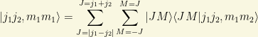
We can relate both sets! The procedure is conceptually (but not analytically, sometimes) simple:

$\displaystyle{\vert j_1j_2,JM\rangle=\sum_{m_1=-j_1}^{j_1}\sum_{m_2=-j_2;m_1+m_2=M}^{j_2}\vert j_1j_2,m_1m_2\rangle\langle j_1j_2,m_1m_2\vert JM\rangle}$

The coefficients:

$\boxed{\langle j_1j_2,m_1m_2\vert JM\rangle}$

are called Clebsch-Gordan coefficients. Moreover, we can also expand the above vectors as follows

$\displaystyle{\vert j_1j_2,m_1m_1\rangle=\sum_{J=\vert j_1-j_2\vert}^{J=j_1+j_2}\sum_{M=-J}^{M=J}\vert J M\rangle \langle J M\vert j_1j_2,m_1m_2\rangle}$

and here the coefficients

$\boxed{\langle J M\vert j_1j_2,m_1m_2\rangle}$

are the inverse Clebsch-Gordan coefficients.

The Clebsch-Gordan coefficients have some beautiful features:

(1) The relative phases are not determined due to the phases in $\vert j_1j_2,JM\rangle$ . They do depend on some coefficients $c_m$ . For any value of J, the phase is determined by recurrence! It shows that

$\langle j_1j_2,j_1 J-j_1\vert J,J\rangle \in \mathbb{R}^+$

This convention implies that the Clebsch-Gordan (CG) coefficients are real numbers and they form an orthogonal matrix!

(2) Selection rules. The CG coefficients $\langle j_1j_2,m_1m_2\vert J,M\rangle$ are necessarily null IF the following conditions are NOT satisfied:

i) $M=m_1+m_2$ .

ii) $\vert j_1-j_2\vert \leq J\leq j_1+j_2$

iii) $j_1+j_2+J\in \mathbb{Z}$

The conditions i) and ii) are trivial. The condition iii) can be obtained from a $2\pi$ rotation to the previous conditions. The two factors that arise are:

$R(2\pi)\vert j,m\rangle=(-1)^{2j}\vert j,m\rangle \leftrightarrow (-1)^{2J}=(-1)^{( j_1+j_2)}$

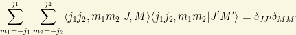
(3) Orthogonality.

$\displaystyle{\sum_{m_1=-j_1}^{j_1}\sum_{m_2=-j_2}^{j_2}\langle j_1j_2,m_1m_2\vert J,M\rangle\langle j_1j_2,m_1m_2\vert J' M'\rangle=\delta_{JJ'}\delta_{MM'}}$

$\displaystyle{\sum_{J=\vert j_1-j_2\vert}^{j_1+j_2}\sum_{M=-J}^{J}\langle j_1j_2,m_1m_2\vert J,M\rangle\langle j_1j_2,m'_1m'_2\vert J M\rangle=\delta_{m_1m'_1}\delta_{m_2m'_2}}$

(4) Minimal/Maximal CG coefficients.

In the case $J,M$ take their minimal/maximal values, the CG are equal to ONE. Check:

$\vert j_1j_2,J=j_1+j_2, J=M\rangle=\vert j_1j_2,m_1=j_1,m_2=j_2\rangle$

(5) Recurrence relations.

5A) First recurrence:

$C_J=\sqrt{J(J+1)-M(M-1)}\langle m_1m_2\vert J,M-1\rangle=$

$=\sqrt{j_1(j_1+1)-m_1(m_1+1)}\langle m_1+1,m_2\vert J,M\rangle+$

$+\sqrt{j_2(j_2+1)-m_2(m_2+1)}\langle m_1,m_2+1\vert J,M\rangle$

5B) Second recurrence:

$C'_J=\sqrt{J(J+1)-M(M+1)}\langle m_1,m_2\vert J,M+1\rangle=$

$=\sqrt{j_1(j_1+1)-m_1(m_1-1)}\langle m_1-1,m_2\vert J,M\rangle+$

$+\sqrt{j_2(j_2+1)-m_2(m_2-1)}\langle m_1,m_2-1\vert J,M\rangle$

These relations 5A) and 5B) are obtained if we apply the ladder operators $J_\pm$ in both sides of the equation defining the CG coefficients and using that

$J_\pm \vert JM\rangle=(J_{1\pm}+J_{2\pm})\vert JM\rangle$

$J_\pm \vert JM\rangle=\hbar \sqrt{J(J+1)-M(M\pm1)}\vert J,M\pm 1\rangle$

Irreducible tensor operators. Wigner-Eckart theorem.

There are 4 important previous definitions for this topic:

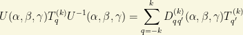
1st. Irreducible Tensor Operator (ITO).

We define $(2k+1)$ operators $T^{(k)}_q$ , with $q\in \left[-k,k\right]$ the standard components of an irreducible tensor operator (ITO) of order $k$ , $T^{(k)}$ , if these components transform according to the following rules

$\displaystyle{U(\alpha,\beta,\gamma)T^{(k)}_qU^{-1}(\alpha,\beta,\gamma)=\sum_{q=-k}^{k}D^{(k)}_{qq'}(\alpha,\beta,\gamma)T^{(k)}_{q'}}$

2nd. Irreducible Tensor Operator (II): commutators.

The $(2k+1)$ operators $T^{(k)}_q$ , $q\in \left[-k,k\right]$ , are the components of an irreducible tensor operator (ITO) of order k, $T^{(k)}$ , if these components satisfy the commutation rules

$\left[J_{\pm},T^{(k)}_q\right]=\hbar \sqrt{k(k+1)-q(q\pm 1)}T^{(k)}_{q\pm 1}$

$\left[ J_z,T^ {(k)}_q\right]=q\hbar T^{(k)}_q$

The 1st and the 2nd definitions are completely equivalent, since the 2nd is the “infinitesimal” version of the 1st. The proof is trivial, by expansion of the operators in series and identification of the involved terms.

3rd. Scalar Operator (SO).

We say that $S=T^0_0$ is an scalar operator, if it is an ITO with order k=0. Equivalently,

$U(\alpha,\beta,\gamma)SU^{-1}(\alpha,\beta,\gamma)=S$

One simple way to express this result is the obvious and natural statement that scalar operators are rotationally invariant!

4th. Vector Operator (VO).

We say that $V$ is a vector operator if

$\displaystyle{U(\alpha,\beta,\gamma)V^{(1)}_qU^{-1}(\alpha,\beta,\gamma)=\sum_{q=-1}^1D^{(1)}_{qq'}(\alpha,\beta,\gamma) V^{(1)}_{q'}}$

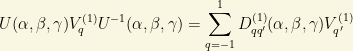
Equivalently, a vector operator is an ITO of order k=1.

The relation between the “standard components” (or “spherical”) and the “cartesian” (i.e.”rectangular”) components is defined by the equations:

$V_1=-\dfrac{1}{2}(V_x+iV_y)$

$V_0=V_z$

$V_{-1}=\dfrac{1}{2}(V_x-iV_y)$

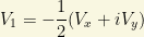
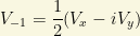
In particular, for the position operator $R=(r_1,r_0,r_{-1})$ , this yields

$r_1=-\dfrac{1}{\sqrt{2}}(x+iy)$

$r_=z$

$r_{-1}=\dfrac{1}{\sqrt{2}}(x-iy)$

Similarly, we can define the components for the momentum operator

$p=(p_1,p_0,p_{-1})$ or the angular momentum

$L=(L_+,L_-,L_z)\equiv (L_1,L_0,L_{-1})$

Now, two questions arise naturally:

1) Consider a set of $(2k+1)(2k'+1)$ operators, built from ITO $T^{(k)}_qT^{(k')}_{q'}$ . Are they ITO too? If not, can they be decomposed into ITO?

2) Consider a set of $(2k+1)(2J+1)$ vectors, built from certain ITO, and a given base of eigenvalues for the angular momentum. Are these vectors an invariant set? Are these vectors an irreducible invariant set? If not, can these vectors be decomposed into irreducible, invariant sets for certain angular momentum operators?

Some theorems help to answer these important questions:

Theorem 1. Consider $T^{(k_1)}_{q_1}, T^{(k_2)}_{q_2}$ , two irreducible tensor operators with $q_1\in \left[-k_1,k_1\right]$ and $q_2\in \left[-k_2,k_2\right]$ . Take $k$ and $q\in \left[-k,k\right]$ arbitrary. Define the quantity

$\displaystyle{S^{(k)}_q\equiv \sum_{q_1=-k_1}^{k_1}\sum_{q_2=-k_2}^{k_2}T^{(k_1)}_{q_1}T^{(k_2)}_{q_2}\langle k_1 k_2,q_1 q_2\vert k q\rangle}$

Then, the operators $S^{(k)}_q$ are the “standard” components of certain ITO with order $k$ . Moreover, we have, using the CG coefficientes:

$\displaystyle{T^{(k_1)}_{q_1}T^{(k_2)}_{q_2}=\sum_{q_1=-k}^{k}\sum_{q_2=\vert k_1-k_2\vert}^{k_1+k_2}S^{(k)}_q\langle k q\vert k_1 k_2, q_1 q_2\rangle}$

Theorem 2. Let $T^{(k)}_{q_1}$ be certain ITO and $\vert j_2 m_1\rangle$ a set of $(2j_2+1)$ eigenvectors of angular momentum. Let us define

$\displaystyle{\vert \omega_{JM }\rangle =\sum_{q_1=-k_1}^{k_1}\sum_{m_2=-j_2}^{j_2}\left(T^{(k_1)}_{q_1}\vert j_2 m_2\rangle\right)\langle k_1 j_2, q_1 m_2\vert J M\rangle}$

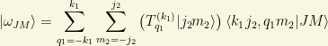
These vectors are eigenvectors of the TOTAL angular momentum:

$J^2\vert \omega_{JM}\rangle =J(J+1)\hbar^2\vert \omega_{JM}\rangle$

$J_z\vert \omega_{JM}\rangle=M\hbar \vert \omega_{JM}\rangle$

Note that, generally, these eigenstates are NOT normalized to the unit, but their moduli do not depend on $M$ . Moreover, using the CG coefficients, we algo get

$\displaystyle{T^{(k)}_{q_1}\vert j_2 m_2\rangle =\sum_{M=-J}^J\sum_{J=\vert k_1-j_2\vert}^{k_1+j_2}\vert J M\rangle \langle J M\vert k_1 j_2, q_1 m_2\rangle}$

Theorem 3 (Wigner-Eckart theorem).

If $T^{(k)}_q$ is an ITO and some bases for angular momentum are provided with $\vert j_1 m_1\rangle$ and $\vert j_2 m_2\rangle$ , then

$\boxed{\langle j_2 m_2\vert T^{(k)}_{q}\vert j_1 m_1\rangle = \langle j_1 j_2, m_1 m_2\vert k q\rangle \dfrac{1}{2k+1}\langle j_2\vert \vert \mathbb{T}^{(k)}_q\vert\vert j_1\rangle}$

and where the quantity

$\boxed{\langle j_2\vert \vert \mathbb{T}^{(k)}_q\vert\vert j_1\rangle}$

is called the reduced matrix element. The proof of this theorem is based on (4) main steps:

1st. Use the $(2k+1)(2j+1)$ vectors (varying $q, m$ ), $T^{(k)}_q\vert j m\rangle$ .

2nd. Form the linear combination/superposition

$\displaystyle{\vert \omega_{JM}\rangle=\sum_{m,q}\left( T^{(k)}_q\vert j m\rangle\right)\langle k j, q m\vert J M\rangle}$

and use the theorem (2) above to obtain

$\langle J' M'\vert J M\rangle=\delta_{JJ}\delta_{MM}F(J)$

3rd. Use the CG coefficients and their properties to rewrite the vectors in the base with J and M. Then, irrespectively the form of the ITO, we obtain

$\displaystyle{T^{(k)}_q\vert j m\rangle=\sum_{J,M}\langle J M\vert k j, q m\rangle \vert \omega_{JM}\rangle}$

4th. Project onto some other different state, we get the desired result

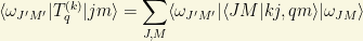
$\displaystyle{\langle \omega_{J'M'}\vert T_q^{(k)}\vert j m\rangle=\sum_{J,M}\langle \omega_{J' M'}\vert \langle J M\vert k j, q m\rangle \vert \omega_{JM}\rangle}$

or equivalently

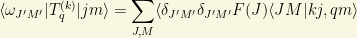
$\displaystyle{\langle \omega_{J'M'}\vert T_q^{(k)}\vert j m\rangle=\sum_{J,M}\langle \delta_{J' M'}\delta_{J'M'}F(J)\langle J M\vert k j,q m\rangle}$

i.e.,

$\displaystyle{\langle \omega_{J'M'}\vert T_q^{(k)}\vert j m\rangle=F(J)\langle J M\vert k j, q m\rangle}$

Q.E.D.

The Wigner-Eckart theorem allows us to determine the so-called selection rules. If you have certain ITO and two bases $\vert j_1,m_1\rangle$ and $\vert j_2, m_2\rangle$ , then we can easily prove from the Wigner-Eckart theorem that

(1) If $m_1-m_1\neq q$ , then $\langle j_1 m_1\vert T^{(k)}_q\vert j_2 m_2\rangle=0$ .

(2) If $\vert j_1-j_2\vert < k < j_1+j_2$ does NOT hold, then $\langle j_1 m_1\vert T^{(k)}_q\vert j_2 m_2\rangle=0$ .

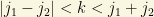
These (selection) rules must be satisfied if some transitions are going to “occur”. There are some “superselection” rules in Quantum Mechanics, an important topic indeed, related to issues like this and symmetry, but this is not the thread where I am going to discuss it! So, stay tuned!

I wish you have enjoyed my basic lectures on group theory!!! Some day I will include more advanced topics, I promise, but you will have to wait with patience, a quality that every scientist should own! 🙂

See you in my next (special) blog post ( number 100!!!!!!!!).

The Spectrum of Riemannium

Physmatics in a nutshell, written and explained by a physmatician. Mobilis in mobili!

Search box

3QD 2012 award

Read/Watch me here too:

Latest posts

Blog subjects

Parallel reading

Papers, talks, data

Spanish Sci-blogs

Extrasolar planets

Technology

Useful software

Science for Everyone

Images from the Universe

Friends

Fun

Free e-books and lectures

Blogroll

My Linux

E-learning

Blog Statistics

Meta stuff

Tags

My twitter account

TSOR (Facebook)

amarashiki