
LOG#074. Dual units.
Posted: 2013/02/03 Filed under: Physmatics, Quantum Gravity, Units, natural units and metrology | Tags: Dual system of units, duality, natural units, speculative ideas 3 CommentsThe last of my three posts tonight is a mysterious dual system of units developed my rival blog (in Spanish language mainly):
http://tardigrados.wordpress.com/
His author launched an interesting but speculative dual system of units in which every physical quantity seems to have a lower and maximal bound. I have never seen such an idea published before, so I translated to English the table he posted here in Spanish language


Is duality the principle/symmetry behind this table? I don’t know for sure, but I came to some similar ideas in my own thoughts about “enhanced relativities”, so I found this table as mysterious as the 
What do you think?
See you soon in a new blog post!
LOG#073. The G2 system.
Posted: 2013/02/03 Filed under: Physmatics, Quantum Gravity, Units, natural units and metrology | Tags: Boya, fundamental units, G2 system, natural units, Rivera, SBR units, sudarshan Leave a commentThe second paper I am going to discuss today is this one:
http://inspirehep.net/record/844954?ln=en
In Note on the natural system of units, Sudarshan, Boya and Rivera introduce a new kind of “fundamental system of units”, that we could call G2 system or the Boya-Rivera-Sudarshan system (BRS system for short). After a summary of the Gamov-Ivanenko-Landau-Okun cube (GILO cube) and the Planck natural units, they make the following question:
Can we change the gravitational constant 
They ask this question due to the fact the 


![\left[G_2\right]=L](https://s0.wp.com/latex.php?latex=%5Cleft%5BG_2%5Cright%5D%3DL&bg=f9f7e1&fg=000000&s=0&c=20201002)
and the physical dimensions of time, length and mass are expressed in terms of 


In fact, they remark that since

and any other equivalent expression to it. Please, note that if we fix the Planck length to unit, we get 
The final remark I would like to make here is that, whatever we choose instead of
See you in my next blog post!
LOG#072. The hG system.
Posted: 2013/02/03 Filed under: Physmatics, Quantum Gravity, Units, natural units and metrology | Tags: charge-mass relationship, compton effect, fundamental theories of physics, fundamental units, G-protocol, h-protocol, hG protocols, hG system, mass pattern, observables Leave a commentBrazil is experimenting an increase of scientific production. Today, I am going to explain this brazilian paper http://arxiv.org/abs/0711.4276v2 concerning the number of fundamental constants.
The Okun cube of fundamental constant, firstly introduced by Gamov, Ivanenko and Landau, has raised some questions about what we should consider as fundamental “unit” we already had but now with more intensity. I mentioned the trialogue of fundamental constants between Veneziano, Duff and Okun himself more than a decade ago. Veneziano argued that 2 fundamental constants were well enought to fix everything. However, it is not the “accepted” and “more popular” approach in these days, but the brazilian paper about defends such a claim!
What do they claim? They basically argue that what we need is a convention for space and time measurements and nothing else. Specifically, they say that every physical observable 

(1)

and where 

After introducing the above statement, they discuss 2 procedures to measure with clocks and rulers, what they call 

(2)

where 
1st. G-protocol. Multiply the above equation (2) by 


i) The unit M from CGS “vanishes” or is “erased” from physical observables.
ii) G disappear from every physical law.
iii) Masses being measured in 


where 


and it has dimensions of 
2nd. h-protocol. From equation (2), if we divide by 


i) M units disappear from physical laws and quantities, as before.
ii) h is erased and vanishes from every equation, law and quantity.
iii) Masses are measured in units of 
and where 


and

The two protocols can be summarized in a nice table
 They also derive the mysterious relations between charge and mass that we saw in the previous post about Pavšič units, i.e., they also derive

and it is equivalent to 
Finally, in their conclusions, they remark that two constants, 


Are 2 fundamental constants enough? Are Veneziano (from a completely different viewpoint) and these brazilian physicists right? Time will tell, but I find interesting these thoughts!
See you soon in another wonderful post about Physmatics and system of units!
LOG#071. Pavšič Units.
Posted: 2013/01/31 Filed under: Physmatics, Units, natural units and metrology | Tags: D-system, dilationally invariant system, Landscape of Theoretical Physics, Matej Pavŝiĉ, natural units 3 CommentsFollowing the thread I began in the previous blog post, today we are going to learn about a non common but very general and universal system of natural units. They were officiallly introduced without name in the literature, until a physicist realized its importance, to my knowledge, by first time.
In his book, The Landscape of Theoretical Physics: A Global View, available here and here for free, the slovenian physicist Matej Pavšič introduced a dilationally invariant system of units, where “all” the fundamental “constants” are set to the unit. More precisely, he defines the D-system or Pavšič units M system characterized by

and where the Coulomb constant 

We have seen in the previous post that addapted system of units do exist where the physical quantities lack any spurious conversion constant (like c or any power or it, the Planck constant and any power of it, and so on). Indeed, we could say that these “fundamental” constants are yet there, but they are “invisible” due to the election of some clever system of units ( the so-called natural units).
The M system of units or D-system ( following M. Pavšič) defines a dilationally invariant system of units, and it is the fact that this system has some special behaviour under “dilatations” why it receives such a name. In the MKSA system, the quantities of this system are written as follows:

We can compare MKSA units and D-system units. Firstly, in MKSA, we have:

However, in D units, we also have:
Of course, this result is the same than the Planck system of units. In addition to these equations, we can also define:


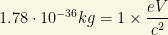
Furthermore, we can also set the electric charge to “mass” as follows (in the D-system):
Length is defined as the radius a classical particle with mass M and a charge elementary e would have. In MKSA, we easily derive:

By the other hand, in terms of units D, it yields

Thus, length seems to be the ratio between “squared charge” and “mass” somehow from D units, i.e., if we further impose that 


in MKSA units, but it is

in D units. Taking the ratio 
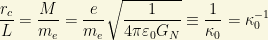
and thus, we can write in D units
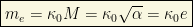
This equation says that mass is equivalent to charge up to a tiny constant, denoted by

This number is roughly 1/295 times the Avogrado constant 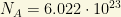

The next table provides the conversion factors between D-system units and MKSA units:

Furthermore, the D units 


Instead of the inhomogeneous coordinates 


For instance, if initially 


If we write a given equation we can check its consistency by comparing the dimension of its left hand and right hand side. In the MKSA system the dimensional control is in checking the powers of meters, kilograms, seconds and ampères on both sides of the equation. Moreover, even the Einstein Field Equations of gravity
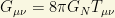
can be expressed in units where 
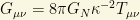
If we choose κ = 1 then the equations for this particular choice correspond to the usual Einstein Field Equations, and we may use either the MKSA system or the D system.
In the D-system, some equations simplify further, even more than in Planck units! Let’s see some interesting uncommon equations in this new system of units:

The final part of this nice post corresponds to a nice exercise included in the Pavšič book. Suppose you are given an equation in the D system, e.g.,

How can we turn it to usual MKSA units? Using conversion constants, we can rewrite the previous equation in the next way:

If we put 1D = 1 then the right hand side of the latter equation is a pure dimensionless quantity. If we wish to obtain a quantity of the dimension of length we have to insert the factor:
and we finally obtain the Böhr radius:

Instead of rewriting equations from the D system in the MKSA system, we can keep all the equations in the D system and perform all the algebraic and numerical calculations in the D units. If we wish to know the numerical results in terms of the MKSA units, we can use the numbers of Table 2 above. For instance, in the previous example, going backwards, we have

Taking D units of length, from Table 1, we read off that 

Let me quote M. Pavšič:
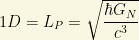
“(…)However, I do not propose to replace the international MKSA system with the D system. I only wish to recall that most modern theoretical works do not use the MKSA system and that it is often very tedious to obtain the results in meters, seconds, kilograms and ampères. (…)besides the Planck length, Planck time and the Planck mass, which are composed of the fundamental constants, 
(or, equivalently, the current and the potential difference), by bringing into play the fundamental constant 


Remarkably, at the end, M. Pavšič points out a classical paper by J.M. Levy-Leblond, see here:http://inspirehep.net/record/128108 , in which, Matej says, is clearly stated that our progress in understanding the unity of nature follows the direction of eliminating from theories various (inessential) numerical constants with the improper name of “fundamental” constants. In fact, those constants are merely the constants which result from our unnatural choice of units, the choice due to our incomplete understanding of the unified theory behind.
Matej Pavšič has become a blogger recently (you can find his site in my links on the right or here) and he has also a nice webpage about his research and lots of interesting topics. He has also studied tachyons, extended objects, geometric algebra, Clifford spaces (C-spaces), brane worlds, relativistic dynamics with an invariant evolution parameter (the so-called Stuckelberg formalism), Kaluza-Klein theories and many other interesting topics. With Carlos Castro Perelman, he is one of the proponents of the theory of relativity in Clifford spaces (C-spaces), an extension of special relativity/general relativity/QFT including grassmann valued quantities and arbitrary signatures on equal footing, but living NOT in spacetime but in some kind of nontrivial and purely algebraic space. You can visit his page and have a look to his works here.
Have you liked this post? Let me know. And be right back for my next communication! Physics is cool, Physmatics is cool and Mathematics is an incredible language for Physmatics!
LOG#070. Natural Units.
Posted: 2013/01/30 Filed under: Classical and Quantum Fields, Cosmology, Gravitational theories, Physmatics, Quantum Gravity, Relativity, The Standard Model: Basics, Units, natural units and metrology | Tags: amount of substance, atomic units, Boltzmann constant, coulomb constant, electric charge, electric current, electric permitivy of vacuum, electromagnetism, ELKO field, Fritzsch-Xing plot, geometrized units, gravitation, gravitational constant, hep units, luminous intensity, mass, mass dimension of fields, MKSA units, mole, natural units, Okun cube, Planck constant, planck units, QCD units, Quantum Gravity, schrödinger units, space, spacetime, speed of light, stoney units, time, TOE, vacuum 1 Comment
Happy New Year 2013 to everyone and everywhere!
Let me apologize, first of all, by my absence… I have been busy, trying to find my path and way in my field, and I am busy yet, but finally I could not resist without a new blog boost… After all, you should know the fact I have enough materials to write many new things.
So, what’s next? I will dedicate some blog posts to discuss a nice topic I began before, talking about a classic paper on the subject here:
https://thespectrumofriemannium.wordpress.com/2012/11/18/log054-barrow-units/
The topic is going to be pretty simple: natural units in Physics.
First of all, let me point out that the election of any system of units is, a priori, totally conventional. You are free to choose any kind of units for physical magnitudes. Of course, that is not very clever if you have to report data, so everyone can realize what you do and report. Scientists have some definitions and popular systems of units that make the process pretty simpler than in the daily life. Then, we need some general conventions about “units”. Indeed, the traditional wisdom is to use the international system of units, or S (Iabbreviated SI from French language: Le Système international d’unités). There, you can find seven fundamental magnitudes and seven fundamental (or “natural”) units:
1) Space:
![\left[ L\right]=\mbox{meter}=m](https://s0.wp.com/latex.php?latex=%5Cleft%5B+L%5Cright%5D%3D%5Cmbox%7Bmeter%7D%3Dm&bg=f9f7e1&fg=000000&s=0&c=20201002)
2) Time:
![\left[ T\right]=\mbox{second}=s](https://s0.wp.com/latex.php?latex=%5Cleft%5B+T%5Cright%5D%3D%5Cmbox%7Bsecond%7D%3Ds&bg=f9f7e1&fg=000000&s=0&c=20201002)
3) Mass:
![\left[ M\right]=\mbox{kilogram}=kg](https://s0.wp.com/latex.php?latex=%5Cleft%5B+M%5Cright%5D%3D%5Cmbox%7Bkilogram%7D%3Dkg&bg=f9f7e1&fg=000000&s=0&c=20201002)
4) Temperature:
![\left[ t\right]=\mbox{Kelvin degree}= K](https://s0.wp.com/latex.php?latex=%5Cleft%5B+t%5Cright%5D%3D%5Cmbox%7BKelvin+degree%7D%3D+K&bg=f9f7e1&fg=000000&s=0&c=20201002)
5) Electric intensity:
![\left[ I\right]=\mbox{ampere}=A](https://s0.wp.com/latex.php?latex=%5Cleft%5B+I%5Cright%5D%3D%5Cmbox%7Bampere%7D%3DA&bg=f9f7e1&fg=000000&s=0&c=20201002)
6) Luminous intensity:
![\left[ I_L\right]=\mbox{candela}=cd](https://s0.wp.com/latex.php?latex=%5Cleft%5B+I_L%5Cright%5D%3D%5Cmbox%7Bcandela%7D%3Dcd&bg=f9f7e1&fg=000000&s=0&c=20201002)
7) Amount of substance:
![\left[ n\right]=\mbox{mole}=mol(e)](https://s0.wp.com/latex.php?latex=%5Cleft%5B+n%5Cright%5D%3D%5Cmbox%7Bmole%7D%3Dmol%28e%29&bg=f9f7e1&fg=000000&s=0&c=20201002)
The dependence between these 7 great units and even their definitions can be found here http://en.wikipedia.org/wiki/International_System_of_Units and references therein. I can not resist to show you the beautiful graph of the 7 wonderful units that this wikipedia article shows you about their “interdependence”:

In Physics, when you build a radical new theory, generally it has the power to introduce a relevant scale or system of units. Specially, the Special Theory of Relativity, and the Quantum Mechanics are such theories. General Relativity and Statistical Physics (Statistical Mechanics) have also intrinsic “universal constants”, or, likely, to be more precise, they allow the introduction of some “more convenient” system of units than those you have ever heard ( metric system, SI, MKS, cgs, …). When I spoke about Barrow units (see previous comment above) in this blog, we realized that dimensionality (both mathematical and “physical”), and fundamental theories are bound to the election of some “simpler” units. Those “simpler” units are what we usually call “natural units”. I am not a big fan of such terminology. It is confusing a little bit. Maybe, it would be more interesting and appropiate to call them “addapted X units” or “scaled X units”, where X denotes “relativistic, quantum,…”. Anyway, the name “natural” is popular and it is likely impossible to change the habits.
In fact, we have to distinguish several “kinds” of natural units. First of all, let me list “fundamental and universal” constants in different theories accepted at current time:
1. Boltzmann constant: 
Essential in Statistical Mechanics, both classical and quantum. It measures “entropy”/”information”. The fundamental equation is:

It provides a link between the microphysics and the macrophysics ( it is the code behind the equation above). It can be understood somehow as a measure of the “energetic content” of an individual particle or state at a given temperature. Common values for this constant are:


Statistical Physics states that there is a minimum unit of entropy or a minimal value of energy at any given temperature. Physical dimensions of this constant are thus entropy, or since 
![\left[ k_B\right] =E/t=J/K](https://s0.wp.com/latex.php?latex=%5Cleft%5B+k_B%5Cright%5D+%3DE%2Ft%3DJ%2FK&bg=f9f7e1&fg=000000&s=0&c=20201002)
2. Speed of light. 
From classical electromagnetism:

The speed of light, according to the postulates of special relativity, is a universal constant. It is frame INDEPENDENT. This fact is at the root of many of the surprising results of special relativity, and it took time to be understood. Moreover, it also connects space and time in a powerful unified formalism, so space and time merge into spacetime, as we do know and we have studied long ago in this blog. The spacetime interval in a D=3+1 dimensional space and two arbitrary events reads:

In fact, you can observe that “c” is the conversion factor between time-like and space-like coordinates. How big the speed of light is? Well, it is a relatively large number from our common and ordinary perception. It is exactly:
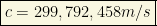
although you often take it as 

and 

![\left[c\right]=LT^{-1}](https://s0.wp.com/latex.php?latex=%5Cleft%5Bc%5Cright%5D%3DLT%5E%7B-1%7D&bg=f9f7e1&fg=000000&s=0&c=20201002)
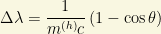
3. Planck’s constant. 
Planck’s constant (or its rationalized version), is the fundamental universal constant in Quantum Physics (Quantum Mechanics, Quantum Field Theory). It gives

Indeed, quanta are the minimal units of energy. That is, you can not divide further a quantum of light, since it is indivisible by definition! Furthermore, the de Broglie relationship relates momentum and wavelength for any particle, and it emerges from the combination of special relativity and the quantum hypothesis:
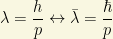
In the case of massive particles, it yields
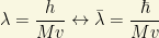
In the case of massless particles (photons, gluons, gravitons,…)


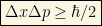
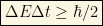
Planck’s constant also appears to be essential to the uncertainty principle of Heisenberg:

Some particularly important values of this constant are:


It is also useful to know that


or


Planck constant has dimension of 

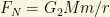
4. Gravitational constant.
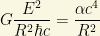
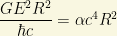
Apparently, it is not like the others but it can also define some particular scale when combined with Special Relativity. Without entering into further details (since I have not discussed General Relativity yet in this blog), we can calculate the escape velocity of a body moving at the speed of light


5. Electric fundamental charge. 
It is generally chosen as fundamental charge the electric charge of the positron (positive charged “electron”). Its value is:

where C denotes Coulomb. Of course, if you know about quarks with a fraction of this charge, you could ask why we prefer this one. Really, it is only a question of hystory of Science, since electrons were discovered first (and positrons). Quarks, with one third or two thirds of this amount of elementary charge, were discovered later, but you could define the fundamental unit of charge as multiple or entire fraction of this charge. Moreover, as far as we know, electrons are “elementary”/”fundamental” entities, so, we can use this charge as unit and we can define quark charges in terms of it too. Electric charge is not a fundamental unit in the SI system of units. Charge flow, or electric current, is.
An amazing property of the above 5 constants is that they are “universal”. And, for instance, energy is related with other magnitudes in theories where the above constants are present in a really wonderful and unified manner:

Caution: k is not the Boltzmann constant but the wave number.
There is a sixth “fundamental” constant related to electromagnetism, but it is also related to the speed of light, the electric charge and the Planck’s constant in a very sutble way. Let me introduce you it too…
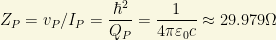
6. Coulomb constant. 
This is a second constant related to classical electromagnetism, like the speed of light in vacuum. Coulomb’s constant, the electric force constant, or the electrostatic constant (denoted

Its experimental value is

Generally, the Coulomb constant is dropped out and it is usually preferred to express everything using the electric permitivity of vacuum 
H.E.P. units
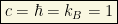
High Energy Physicists use to employ units in which the velocity is measured in fractions of the speed of light in vacuum, and the action/angular momentum is some multiple of the Planck’s constant. These conditions are equivalent to set


Complementarily, or not, depending on your tastes and preferences, you can also set the Boltzmann’s constant to the unit as well

and thus the complete HEP system is defined if you set
This “natural” system of units is lacking yet a scale of energy. Then, it is generally added the electron-volt 
This system of units have remarkable conversion factors
A) 
B) 
C)

D)
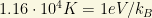
E) 
F)

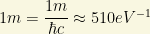
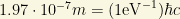
This system of units, therefore, leaves free only the energy scale (generally it is chosen the electron-volt) and the electric measure of fundamentl charge. Every other unit can be related to energy/charge. It is truly remarkable than doing this (turning invisible the above three constants) you can “unify” different magnitudes due to the fact these conventions make them equivalent. For instance, with natural units:
1) Length=Time=1/Energy=1/Mass.
It is due to 


Note that natural units turn invisible the units we set to the unit! That is the key of the procedure. It simplifies equations and expressions. Of course, you must be careful when you reintroduce constants!
2) Energy=Mass=Momemntum=Temperature.
It is due to 

One extra bonus for theoretical physicists is that natural units allow to build and write proper lagrangians and hamiltonians (certain mathematical operators containing the dynamics of the system enconded in them), or equivalently the action functional, with only the energy or “mass” dimension as “free parameter”. Let me show how it works.
Natural units in HEP identify length and time dimensions. Thus ![\left[L\right]=\left[T\right]](https://s0.wp.com/latex.php?latex=%5Cleft%5BL%5Cright%5D%3D%5Cleft%5BT%5Cright%5D&bg=f9f7e1&fg=000000&s=0&c=20201002)
![\boxed{\left[L\right]=\left[T\right]=\left[E\right]^{-1}}](https://s0.wp.com/latex.php?latex=%5Cboxed%7B%5Cleft%5BL%5Cright%5D%3D%5Cleft%5BT%5Cright%5D%3D%5Cleft%5BE%5Cright%5D%5E%7B-1%7D%7D&bg=f9f7e1&fg=000000&s=0&c=20201002)
The speed of light identifies energy and mass, and thus, we can often heard about “mass-dimension” of a lagrangian in the following sense. HEP units can be thought as defining “everything” in terms of energy, from the pure dimensional ground. That is, every physical dimension is (in HEP units) defined by a power of energy:
![\boxed{\left[E\right]^n}](https://s0.wp.com/latex.php?latex=%5Cboxed%7B%5Cleft%5BE%5Cright%5D%5En%7D&bg=f9f7e1&fg=000000&s=0&c=20201002)
Thus, we can refer to any magnitude simply saying the power of such physical dimension (or you can think logarithmically to understand it easier if you wish). With this convention, and recalling that energy dimension is mass dimension, we have that
![\left[L\right]=\left[T\right]=-1](https://s0.wp.com/latex.php?latex=%5Cleft%5BL%5Cright%5D%3D%5Cleft%5BT%5Cright%5D%3D-1&bg=f9f7e1&fg=000000&s=0&c=20201002)
![\left[E\right]=\left[M\right]=1](https://s0.wp.com/latex.php?latex=%5Cleft%5BE%5Cright%5D%3D%5Cleft%5BM%5Cright%5D%3D1&bg=f9f7e1&fg=000000&s=0&c=20201002)
Using these arguments, the action functional is a pure dimensionless quantity, and thus, in D=4 spacetime dimensions, lagrangian densities must have dimension 4 ( or dimension D is a general spacetime).
![\displaystyle{S=\int d^4x \mathcal{L}\rightarrow \left[\mathcal{L}\right]=4}](https://s0.wp.com/latex.php?latex=%5Cdisplaystyle%7BS%3D%5Cint+d%5E4x+%5Cmathcal%7BL%7D%5Crightarrow+%5Cleft%5B%5Cmathcal%7BL%7D%5Cright%5D%3D4%7D&bg=f9f7e1&fg=000000&s=0&c=20201002)
![\displaystyle{S=\int d^Dx \mathcal{L}\rightarrow \left[\mathcal{L}\right]=D}](https://s0.wp.com/latex.php?latex=%5Cdisplaystyle%7BS%3D%5Cint+d%5EDx+%5Cmathcal%7BL%7D%5Crightarrow+%5Cleft%5B%5Cmathcal%7BL%7D%5Cright%5D%3DD%7D&bg=f9f7e1&fg=000000&s=0&c=20201002)
In D=4 spacetime dimensions, it can be easily showed that
![\left[\partial_\mu\right]=\left[\Phi\right]=\left[A^\mu\right]=1](https://s0.wp.com/latex.php?latex=%5Cleft%5B%5Cpartial_%5Cmu%5Cright%5D%3D%5Cleft%5B%5CPhi%5Cright%5D%3D%5Cleft%5BA%5E%5Cmu%5Cright%5D%3D1&bg=f9f7e1&fg=000000&s=0&c=20201002)
![\left[\Psi_D\right]=\left[\Psi_M\right]=\left[\chi\right]=\left[\eta\right]=\dfrac{3}{2}](https://s0.wp.com/latex.php?latex=%5Cleft%5B%5CPsi_D%5Cright%5D%3D%5Cleft%5B%5CPsi_M%5Cright%5D%3D%5Cleft%5B%5Cchi%5Cright%5D%3D%5Cleft%5B%5Ceta%5Cright%5D%3D%5Cdfrac%7B3%7D%7B2%7D&bg=f9f7e1&fg=000000&s=0&c=20201002)
where 


![\boxed{\left[\Phi\right]=\left[A_\mu\right]=\dfrac{D-2}{2}\equiv E^{\frac{D-2}{2}}=M^{\frac{D-2}{2}}}](https://s0.wp.com/latex.php?latex=%5Cboxed%7B%5Cleft%5B%5CPhi%5Cright%5D%3D%5Cleft%5BA_%5Cmu%5Cright%5D%3D%5Cdfrac%7BD-2%7D%7B2%7D%5Cequiv+E%5E%7B%5Cfrac%7BD-2%7D%7B2%7D%7D%3DM%5E%7B%5Cfrac%7BD-2%7D%7B2%7D%7D%7D&bg=f9f7e1&fg=000000&s=0&c=20201002)
![\boxed{\left[\Psi\right]=\dfrac{D-1}{2}\equiv E^{\frac{D-1}{2}}=M^{\frac{D-1}{2}}}](https://s0.wp.com/latex.php?latex=%5Cboxed%7B%5Cleft%5B%5CPsi%5Cright%5D%3D%5Cdfrac%7BD-1%7D%7B2%7D%5Cequiv+E%5E%7B%5Cfrac%7BD-1%7D%7B2%7D%7D%3DM%5E%7B%5Cfrac%7BD-1%7D%7B2%7D%7D%7D&bg=f9f7e1&fg=000000&s=0&c=20201002)
Remark (for QFT experts only): Don’t confuse mass dimension with the final transverse polarization degrees or “degrees of freedom” of a particular field, i.e., “components” minus “gauge constraints”. E.g.: a gauge vector field has 
In summary:
i) HEP units are based on QM (Quantum Mechanics), SR (Special Relativity) and Statistical Mechanics (Entropy and Thermodynamics).
ii) HEP units need to introduce a free energy scale, and it generally drives us to use the eV or electron-volt as auxiliary energy scale.
iii) HEP units are useful to dimensional analysis of lagrangians (and hamiltonians) up to “mass dimension”.
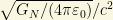
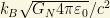
Stoney Units
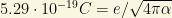
In Physics, the Stoney units form a alternative set of natural units named after the Irish physicist George Johnstone Stoney, who first introduced them as we know it today in 1881. However, he presented the idea in a lecture entitled “On the Physical Units of Nature” delivered to the British Association before that date, in 1874. They are the first historical example of natural units and “unification scale” somehow. Stoney units are rarely used in modern physics for calculations, but they are of historical interest but some people like Wilczek has written about them (see, e.g., http://arxiv.org/abs/0708.4361). These units of measurement were designed so that certain fundamental physical constants are taken as reference basis without the Planck scale being explicit, quite a remarkable fact! The set of constants that Stoney used as base units is the following:
A) Electric charge, 
B) Speed of light in vacuum, 
C) Gravitational constant, 
D) The Reciprocal of Coulomb constant, 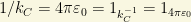
Stony units are built when you set these four constants to the unit, i.e., equivalently, the Stoney System of Units (S) is determined by the assignments:
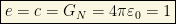
Interestingly, in this system of units, the Planck constant is not equal to the unit and it is not “fundamental” (Wilczek remarked this fact here ) but:

Today, Planck units are more popular Planck than Stoney units in modern physics, and even there are many physicists who don’t know about the Stoney Units! In fact, Stoney was one of the first scientists to understand that electric charge was quantized!; from this quantization he deduced the units that are now named after him.
The Stoney length and the Stoney energy are collectively called the Stoney scale, and they are not far from the Planck length and the Planck energy, the Planck scale. The Stoney scale and the Planck scale are the length and energy scales at which quantum processes and gravity occur together. At these scales, a unified theory of physics is thus likely required. The only notable attempt to construct such a theory from the Stoney scale was that of H. Weyl, who associated a gravitational unit of charge with the Stoney length and who appears to have inspired Dirac’s fascination with the large number hypothesis. Since then, the Stoney scale has been largely neglected in the development of modern physics, although it is occasionally discussed to this day. Wilczek likes to point out that, in Stoney Units, QM would be an emergent phenomenon/theory, since the Planck constant wouldn’t be present directly but as a combination of different constants. By the other hand, the Planck scale is valid for all known interactions, and does not give prominence to the electromagnetic interaction, as the Stoney scale does. That is, in Stoney Units, both gravitation and electromagnetism are on equal footing, unlike the Planck units, where only the speed of light is used and there is no more connections to electromagnetism, at least, in a clean way like the Stoney Units do. Be aware, sometimes, rarely though, Planck units are referred to as Planck-Stoney units.
What are the most interesting Stoney system values? Here you are the most remarkable results:
1) Stoney Length, 

2) Stoney Mass, 

3) Stoney Energy, 

4) Stoney Time, 
5) Stoney Charge, 

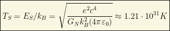
6) Stoney Temperature, 
Planck Units
The reference constants to this natural system of units (generally denoted by P) are the following 4 constants:
1) Gravitational constant.
2) Speed of light.
3) Planck constant or rationalized Planck constant.
4) Boltzmann constant.
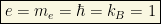
The Planck units are got when you set these 4 constants to the unit, i.e.,

It is often said that Planck units are a system of natural units that is not defined in terms of properties of any prototype, physical object, or even features of any fundamental particle. They only refer to the basic structure of the laws of physics: c and G are part of the structure of classical spacetime in the relativistic theory of gravitation, also known as general relativity, and ℏ captures the relationship between energy and frequency which is at the foundation of elementary quantum mechanics. This is the reason why Planck units particularly useful and common in theories of quantum gravity, including string theory or loop quantum gravity.
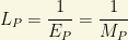
This system defines some limit magnitudes, as follows:
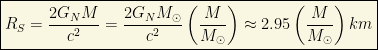
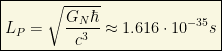
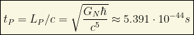
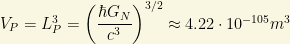
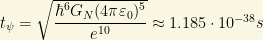
1) Planck Length, 
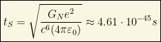
2) Planck Time, 
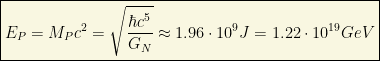
3) Planck Mass, 

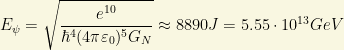
4) Planck Energy, 
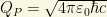
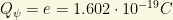
5) Planck charge, 
In Lorentz-Heaviside electromagnetic units

In Gaussian electromagnetic units

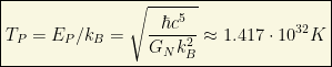
6) Planck temperature, 
From these “fundamental” magnitudes we can build many derived quantities in the Planck System:
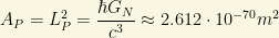
1) Planck area.
2) Planck volume.
3) Planck momentum.

A relatively “small” momentum!
4) Planck force.
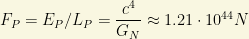
It is independent from Planck constant! Moreover, the Planck acceleration is

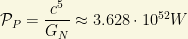
5) Planck Power.
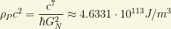
6) Planck density.
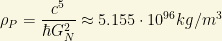
Planck density energy would be equal to
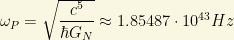
7) Planck angular frequency.
8) Planck pressure.

Note that Planck pressure IS the Planck density energy!
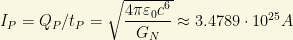
9) Planck current.
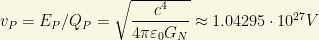
10) Planck voltage.
11) Planck impedance.
A relatively small impedance!
12) Planck capacitor.

Interestingly, it depends on the gravitational constant!
Some Planck units are suitable for measuring quantities that are familiar from daily experience. In particular:
1 Planck mass is about 22 micrograms.
1 Planck momentum is about 6.5 kg m/s
1 Planck energy is about 500kWh.
1 Planck charge is about 11 elementary (electronic) charges.
1 Planck impendance is almost 30 ohms.
Moreover:
i) A speed of 1 Planck length per Planck time is the speed of light, the maximum possible speed in special relativity.
ii) To understand the Planck Era and “before” (if it has sense), supposing QM holds yet there, we need a quantum theory of gravity to be available there. There is no such a theory though, right now. Therefore, we have to wait if these ideas are right or not.
iii) It is believed that at Planck temperature, the whole symmetry of the Universe was “perfect” in the sense the four fundamental foces were “unified” somehow. We have only some vague notios about how that theory of everything (TOE) would be.
The physical dimensions of the known Universe in terms of Planck units are “dramatic”:
i) Age of the Universe is about 
ii) Diameter of the observable Universe is about

iii) Current temperature of the Universe is about

iv) The observed cosmological constant is about

v) The mass of the Universe is about 
vi) The Hubble constant is

Schrödinger Units
The Schrödinger Units do not obviously contain the term c, the speed of light in a vacuum. However, within the term of the Permittivity of Free Space [i.e., electric constant or vacuum permittivity], and the speed of light plays a part in that particular computation. The vacuum permittivity results from the reciprocal of the speed of light squared times the magnetic constant. So, even though the speed of light is not apparent in the Schrödinger equations it does exist buried within its terms and therefore influences the decimal placement issue within square roots. The essence of Schrödinger units are the following constants:
A) Gravitational constant
B) Planck constant
C) Boltzmann constant
D) Coulomb constant or equivalently the electric permitivity of free space/vacuum
E) The electric charge of the positron
In this sistem 
1) Schrödinger Length 
2) Schrödinger time 
3) Schrödinger mass 

4) Schrödinger energy 
5) Schrödinger charge 
6) Schrödinger temperature 

Atomic Units
There are two alternative systems of atomic units, closely related:
1) Hartree atomic units:

2) Rydberg atomic units:


There, 

The units are adapted to characterize the behavior of an electron in the ground state of a hydrogen atom. For example, using the Hartree convention, in the Böhr model of the hydrogen atom, an electron in the ground state has orbital velocity = 1, orbital radius = 1, angular momentum = 1, ionization energy equal to 1/2, and so on.
Some quantities in the Hartree system of units are:
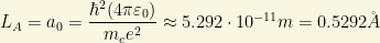
1) Atomic Length (also called Böhr radius):
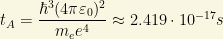
2) Atomic Time:
3) Atomic Mass:

4) Atomic Energy:

5) Atomic electric Charge:

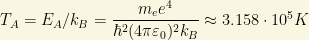
6) Atomic temperature:
The fundamental unit of energy is called the Hartree energy in the Hartree system and the Rydberg energy in the Rydberg system. They differ by a factor of 2. The speed of light is relatively large in atomic units (137 in Hartree or 274 in Rydberg), which comes from the fact that an electron in hydrogen tends to move much slower than the speed of light. The gravitational constant is extremely small in atomic units (about 10−45), which comes from the fact that the gravitational force between two electrons is far weaker than the Coulomb force . The unit length, LA, is the so-called and well known Böhr radius, a0.
The values of c and e shown above imply that 
QCD Units
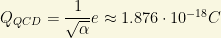
In the framework of Quantum Chromodynamics, a quantum field theory (QFT) we know as QCD, we can define the QCD system of units based on:
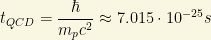
1) QCD Length 

and where 
2) QCD Time 
3) QCD Mass 

4) QCD Energy 

Thus, QCD energy is about 1 GeV!
5) QCD Temperature 

6) QCD Charge 
In Heaviside-Lorent units:

In Gaussian units:
Geometrized Units
The geometrized unit system, used in general relativity, is not a completely defined system. In this system, the base physical units are chosen so that the speed of light and the gravitational constant are set equal to unity. Other units may be treated however desired. By normalizing appropriate other units, geometrized units become identical to Planck units. That is, we set:

and the remaining constants are set to the unit according to your needs and tastes.
Conversion Factors
This table from wikipedia is very useful:

where:
i)
ii) 
Some conversion factors for geometrized units are also available:
Conversion from kg, s, C, K into m:


Conversion from m, s, C, K into kg:


Conversion from m, kg, C, K into s


Conversion from m, kg, s, K into C


Conversion from m, kg, s, C into K


Or you can read off factors from this table as well:

and

Advantages and Disadvantages of Natural Units
Natural units have some advantages (“Pro”):
1) Equations and mathematical expressions are simpler in Natural Units.
2) Natural units allow for the match between apparently different physical magnitudes.
3) Some natural units are independent from “prototypes” or “external patterns” beyond some clever and trivial conventions.
4) They can help to unify different physical concetps.
However, natural units have also some disadvantages (“Cons”):
1) They generally provide less precise measurements or quantities.
2) They can be ill-defined/redundant and own some ambiguity. It is also caused by the fact that some natural units differ by numerical factors of pi and/or pure numbers, so they can not help us to understand the origin of some pure numbers (adimensional prefactors) in general.
Moreover, you must not forget that natural units are “human” in the sense you can addapt them to your own needs, and indeed,you can create your own particular system of natural units! However, said this, you can understand the main key point: fundamental theories are who finally hint what “numbers”/”magnitudes” determine a system of “natural units”.
Remark: the smart designer of a system of natural unit systems must choose a few of these constants to normalize (set equal to 1). It is not possible to normalize just any set of constants. For example, the mass of a proton and the mass of an electron cannot both be normalized: if the mass of an electron is defined to be 1, then the mass of a proton has to be 

where
Fritzsch-Xing plot
Fritzsch and Xing have developed a very beautiful plot of the fundamental constants in Nature (those coming from gravitation and the Standard Model). I can not avoid to include it here in the 2 versions I have seen it. The first one is “serious”, with 29 “fundamental constants”:

However, I prefer the “fun version” of this plot. This second version is very cool and it includes 28 “fundamental constants”:

The Okun Cube
Long ago, L.B. Okun provided a very interesting way to think about the Planck units and their meaning, at least from current knowledge of physics! He imagined a cube in 3d in which we have 3 different axis. Planck units are defined as we have seen above by 3 constants 

Or equivalently, sometimes it is seen as an equivalent sketch ( note the Planck constant is NOT rationalized in the next cube, but it does not matter for this graphical representation):

Classical physics (CP) corresponds to the vanishing of the 3 constants, i.e., to the origin 
Newtonian mechanics (NM) , or more precisely newtonian gravity plus classical mechanics, corresponds to the “point” 
Special relativity (SR) corresponds to the point 
Quantum mechanics (QM) corresponds to the point 
Quantum Field Theory (QFT) corresponds to the point 
Quantum Gravity (QG) would correspond to the point 
Finally, the Theory Of Everything (TOE) would be the theory in the last free corner, that arising in the vertex 
Some final remarks and questions
1) Are fundamental “constants” really constant? Do they vary with energy or time?
2) How many fundamental constants are there? This questions has provided lots of discussions. One of the most famous was this one:
http://arxiv.org/abs/physics/0110060
The trialogue (or dialogue if you are precise with words) above discussed the opinions by 3 eminent physicists about the number of fundamental constants: Michael Duff suggested zero, Gabriel Veneziano argued that there are only 2 fundamental constants while L.B. Okun defended there are 3 fundamental constants
3) Should the cosmological constant be included as a new fundamental constant? The cosmological constant behaves as a constant from current cosmological measurements and cosmological data fits, but is it truly constant? It seems to be…But we are not sure. Quintessence models (some of them related to inflationary Universes) suggest that it could vary on cosmological scales very slowly. However, the data strongly suggest that

It is simple, but it is not understood the ultimate nature of such a “fluid” because we don’t know what kind of “stuff” (either particles or fields) can make the cosmological constant be so tiny and so abundant (about the 72% of the Universe is “dark energy”/cosmological constant) as it seems to be. We do know it can not be “known particles”. Dark energy behaves as a repulsive force, some kind of pressure/antigravitation on cosmological scales. We suspect it could be some kind of scalar field but there are many other alternatives that “mimic” a cosmological constant. If we identify the cosmological constant with the vacuum energy we obtain about 122 orders of magnitude of mismatch between theory and observations. A really bad “prediction”, one of the worst predictions in the history of physics!
Be natural and stay tuned!
LOG#054. Barrow units.
Posted: 2012/11/18 Filed under: Physmatics, Units, natural units and metrology 3 CommentsIn a nice paper titled Dimensionality, see here http://rsta.royalsocietypublishing.org/content/310/1512/337.short , the physicist John Barrow studied the rôle of known fundamental constants and their links to the dimensionality of space-time.
I will review the main ideas appearing in that paper, and some interesting conclusions we can obtain from it.
Firstly, Barrow points out the connection between some equations and dimensionality. For instance, the Poisson-Laplace equation in any dimension 

and a force

whenever spherical symmetry holds 

The atomic stability can be read from a really simple condition for the energy with a Coulomb potential:
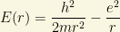
Imposing 

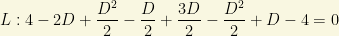
Indeed, Ehrenfest proved that for atoms in 


This fact means that only 3d space (4D spacetime) appears to have the beautiful and nice properties necessary for transmissions of high fidelity signal due to the simultaneous realization of reverberationless and distortionless propagation of information.
Barrow realized that we can build a dimensionless basic and fundamental system of units, that we can call Barrow units system (or Barrow system). The dimensionless quantity of this system is made of 4 constants:
1st. The electric charge
Its physical units are ![\left[ e^2\right]=ML^DT^{-2}](https://s0.wp.com/latex.php?latex=%5Cleft%5B+e%5E2%5Cright%5D%3DML%5EDT%5E%7B-2%7D&bg=f9f7e1&fg=000000&s=0&c=20201002)
![\left[ e\right]=M^{1/2}L^{D/2}T^{-1}](https://s0.wp.com/latex.php?latex=%5Cleft%5B+e%5Cright%5D%3DM%5E%7B1%2F2%7DL%5E%7BD%2F2%7DT%5E%7B-1%7D&bg=f9f7e1&fg=000000&s=0&c=20201002)
2nd. The Planck constant
Its physical units are
![\left[ \hbar\right]=ML^2T^{-1}](https://s0.wp.com/latex.php?latex=%5Cleft%5B+%5Chbar%5Cright%5D%3DML%5E2T%5E%7B-1%7D&bg=f9f7e1&fg=000000&s=0&c=20201002)
3rd. The Newton gravitational constant
Its physical units are
![\left[ G_N\right]=M^{-1}L^DT^{-2}](https://s0.wp.com/latex.php?latex=%5Cleft%5B+G_N%5Cright%5D%3DM%5E%7B-1%7DL%5EDT%5E%7B-2%7D&bg=f9f7e1&fg=000000&s=0&c=20201002)
4th. The speed of light
Its physical units are
![\left[ c\right]=LT^{-1}](https://s0.wp.com/latex.php?latex=%5Cleft%5B+c%5Cright%5D%3DLT%5E%7B-1%7D&bg=f9f7e1&fg=000000&s=0&c=20201002)
From these 4 fundamental constants, the Barrow system formed by 

Remarks:
1) 
i) The electric charge/electromagnetic coupling constant in D=1.

ii) Planck’s constant/The quantum theory fundamental constant in D=2.

iii) Gravitational Newton constant/gravitational Newton coupling constant in D=3.

iv) The speed of light/The fundamental constant of special relativity in D=4.

2) Dimensionless units for all 
3) Fractal dimensions with non-integer values are not allowed in this classical setting. We note that strange attractors provide objects with non-integer dimensions 
4) A fundamental length L can emerge from quantum gravity (QG). In the most general case, it would imply

where 


From special relativity 

Therefore,

We introduce 


Q.E.D.
5) Fractal dimension theory will not be considered in this post, but it deserves further study.
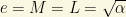
6) We will check that the dimensionless fundamental constant for the Barrow system is 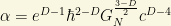

Thus, for M, L and T, we deduce:


Q.E.D.


You must be logged in to post a comment.