
LOG#127. Basic Neutrinology(XII).
Posted: 2013/07/22 Filed under: Basic Neutrinology, Physmatics | Tags: electron density, mass eigenstates, matter density, MSW effect, neutrino mixing, neutrino oscillations, neutrino oscillations in matter, neutrino oscillatrions in vacuum, neutrino refraction, neutrinology, refraction, resonance, weak eigenstates Leave a comment
When neutrinos pass through matter or they propagate in a medium (not in the vacuum), a subtle and potentially important effect occurs. This is called the MSW effect (Mikheyev-Smirnov-Wolfenstein effect). It is pretty similar to a refraction of light in a medium, but now it happens that the particle (wave) propagating are not electromagnetic waves (photons) but neutrinos! In fact, the MSW effect consists in two different effects:
1st. A “resonance” enhancement of the neutrino oscillation pattern.
2nd. An adiabatic (i.e. slow) or partially adiabatic neutrino conversion (mixing).
In the presence of matter, the neutrino experiences scattering and absorption. This last phenomenon is always negligible (or almost in most cases). At very low energies, coherent elastic forward scattering is the most important process. Similarly to optics, the net effect is the appearance of a phase difference, a refractive index or, equivalently, a neutrino effective mass.
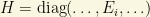
The neutrino effective mass can cause an important change in the neutrino oscillation pattern, depending on the densities and composition of the medium. It also depends on the nature of the neutrino (its energy, its type and its oscillation length). In the neutrino case, the medium is “flavor-dispersive”: the matter is usually non-symmetric with respect to the lepton numbers! Then, the effective neutrino mass is different for the different weak eigenstates!
I will try to explain it as simple as possible here. For instance, take the solar electron plasma. The electrons in the solar medium have charged current interactions with 

(1)
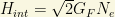
where the numerical prefactor is conventional, 

(2)
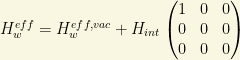
The consequence of this new effective hamiltonian is that the oscillation probabilities of the neutrino in matter can be largely increased due to a resonance with matter. In matter, for the simplest case with 2 flavors and 2 dimensions, we can define an effective oscillation/mixing angle as
(3)
![\boxed{\sin\theta_M=\dfrac{\sin 2\theta/L_{osc}}{\left[\left(\cos 2\theta/L_{osc}-G_FN_e/\sqrt{2}\right)^2+\left(\sin 2\theta/L_{osc}\right)^2\right]^{1/2}}}](https://s0.wp.com/latex.php?latex=%5Cboxed%7B%5Csin%5Ctheta_M%3D%5Cdfrac%7B%5Csin+2%5Ctheta%2FL_%7Bosc%7D%7D%7B%5Cleft%5B%5Cleft%28%5Ccos+2%5Ctheta%2FL_%7Bosc%7D-G_FN_e%2F%5Csqrt%7B2%7D%5Cright%29%5E2%2B%5Cleft%28%5Csin+2%5Ctheta%2FL_%7Bosc%7D%5Cright%29%5E2%5Cright%5D%5E%7B1%2F2%7D%7D%7D&bg=f9f7e1&fg=000000&s=0&c=20201002)
The presence of the term proportional to the electron density can produce “a resonance” nullifying the denominator. there is a critical density 
(3)
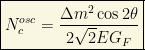
for which the matter mixing angle 


1st.
2nd. The kinematical factor differs by the replacement of 

(4)
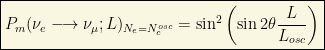
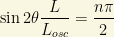
This equation tells us that we can get a full conversion of electron neutrino weak eigenstates into muon weak eigenstates, provided that the length and energy of the neutrino satisfy the condition
There is a second interesting limit that is mentioned often. This limit happens whenever the electron density 


Therefore, the lesson here is that a big density can spoil the phenomenon of neutrino oscillations!
In summary, we have learned here that:
1st. There are neutrino oscillations “triggered” by matter. Matter can enhance or enlarge neutrino mixing by “resonance”.
2nd. A high enough matter density can spoil the neutrino mixing (the complementary effect to the previous one).
The MSW effect is particularly important in the field of geoneutrinos and when the neutrinos pass through the Earth core or mantle, as much as it also matters inside the stars or in collapsing stars that will become into supernovae. The flavor of neutrino states follows changes in the matter density!
See you in my next neutrinological post!
LOG#126. Basic Neutrinology(XI).
Posted: 2013/07/22 Filed under: Basic Neutrinology, Physmatics, The Standard Model: Basics | Tags: IceCube, LBE, long baseline experiments, neutrino beam experiments, neutrino masses and lepton asymmetry, neutrino mixing, neutrino oscillation experiments, neutrino oscillations, neutrino oscillations in matter, neutrino oscillations in vacuum, neutrino telescopes, neutrinology, NOCILLA, NOSEX, reactor experiments, right-handed neutrinos, SBE, short baseline experiments, sterile neutrinos Leave a comment
Why is the case of massive neutrinos so relevant in contemporary physics? The full answer to this question would be very long. In fact, I am making this long thread about neutrinology in order you understand it a little bit. If neutrinos do have nonzero masses, then, due to the basic postulates of the quantum theory there will be in a “linear combination” or “mixing” among all the possible “states”. It also happens with quarks! This mixing will be observable even at macroscopic distances from the production point or source and it has very important practical consequences ONLY if the difference of the neutrino masses squared are very small. Mathematically speaking 

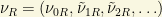
In the presence of neutrino masses, the so-called “weak eigenstates” are different to “mass eigenstates”. There is a “transformation” or “mixing”/”oscillation” between them. This phenomenon is described by some unitary matrix U. The idea is:


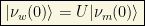
If neutrinos can only be created and detected as a result of weak processes, at origin (or any arbitrary point) we have a weak eigenstate as a “rotation” of a mass eigenstate through the mixing matrix U:
In this post, I am only to introduce the elementary theory of neutrino oscillations (NO or NOCILLA)/neutrino mixing (NOMIX) from a purely heuristic viewpoint. I will be using natural units with 
If we ignore the effects of the neutrino spin, after some time the system will evolve into the next state (recall we use elementary hamiltonian evolution from quantum mechanics here):

and where 
and here, using special relativity, we write

In most of the interesting cases (when 


The effective neutrino hamiltonian can be written as

and

In this last equation, we write

with

We can perform this derivation in a more rigorous mathematical structure, but I am not going to do it here today. The resulting theory of neutrino mixing and neutrino oscillations (NO) has a beautiful corresponded with Neutrino OScillation EXperiments (NOSEX). These experiments are usually analyzed under the simplest assumption of two flavor mixing, or equivalently, under the perspective of neutrino oscillations with 2 simple neutrino species we can understand this process better. In such a case, the neutrino mixing matrix U becomes a simple 2-dimensional orthogonal rotation matrix depending on a single parameter 


(1)
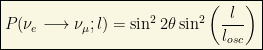
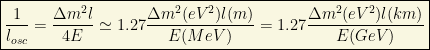
This important formula describes the probability of NO in the 2-flavor case. It is a very important and useful result! There, we have defined the oscillation length as

with 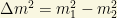
(2)
As you can observe, the probabilities depend on two factors: the mixing (oscillation) angle and the kinematical factor as a function of the traveled distance, the momentum of the neutrinos and the mass difference between the two species. If this mass difference were probed to be non-existent, the phenomenon of the neutrino oscillation would not be possible (it would have 0 probability!). To observe the neutrino oscillation, we have to make (observe) neutrinos in which some of this parameters are “big”, so the probability is significant. Interestingly, we can have different kind of neutrino oscillation experiments according to how large are these parameters. Namely:
–Long baseline experiments (LBE). This class of NOSEX happen whenever you have an oscillation length of order 
-Short baseline experiments (SBE). This class of NOSEX happen whenever the distances than neutrino travel are lesser than hundreds of kilometers, perhaps some. Of course, the issue is conventional. Reactor experiments like KamLAND in Japan (Daya Bay in China, or RENO in South Korea) are experiments of this type.
Moreover, beyond reactor experiments, you also have neutrino beam experiments (T2K, 
In summary, the phenomenon of neutrino mixing/neutrino oscillations/changing neutrino flavor transforms the neutrino in a very special particle under quantum and relativistic theories. Neutrinos are one of the best tools or probes to study matter since they only interact under weak interactions and gravity! Therefore, neutrinos are a powerful “laboratory” in which we can test or search for new physics (The fact that neutrinos are massive is, said this, a proof of new physics beyond the SM since the SM neutrinos are massless!). Indeed, the phenomenon is purely quantum and (special) relativist since the neutrinos are tiny particles and “very fast”. We have seen what are the main ideas behind this phenomenon and the main classes of neutrino experiments (long baseline and shortbaseline experiments). Moreover, we also have “passive” neutrino detectors like SuperKamiokande, IceCube and many others I will not quote here. They study the neutrino oscillations detecting atmospheric neutrinos (the result of cosmic rays hitting the atmosphere), solar neutrinos and other astrophysical sources of neutrinos (like supernovae!). I have talked you about cosmic relic neutrinos too in the previous post. Aren’t you convinced that neutrinos are cool? They are “metamorphic”, they have flavor, they are everywhere!
See you in my next neutrinological post!
LOG#125. Basic Neutrinology(X).
Posted: 2013/07/17 Filed under: Basic Neutrinology, Physmatics, The Standard Model: Basics | Tags: 5 sigma, CMB, CNB, cosmic ray, cosmic rays and physics, cross-section, delta particle, delta resonance, Greisen–Zatsepin–Kuzmin limit, GZK cut-off, GZK effect, H-burst, H-dip, neutrino astronomy, neutrino cosmology, neutrino spectroscopy, neutrinology, resonance, X-burst, X-dip, Z-burst, Z-dip, Zetta-electron-volt, ZeV, Zevatron Leave a comment
The topic today is a fascinant subject in Neutrino Astronomy/Astrophysics/Cosmology. I have talked you in this thread about the cosmic neutrino background (
1st. If we want to study the early Universe, we need some “new” tool to overcome the last scattering surface as a consequence of the Cosmic Microwave Background (CMB). Neutrinos are such a new tool/probe! They only interact weakly with matter and we suspect that there are some important pieces of information related to the quark and lepton “complementarity” hidden in their mixing parameters.
2nd. Due to the GZK effect, we expect that the flux of cosmic rays will suffer a sudden cut-off at about 


The limit is at the same order of magnitude as the upper limit for energy at which cosmic rays have experimentally been detected. There are some current experiments that “claim” to have observed this GZK effect, but evidence is not conclusive yet as far as I know. Some experiments claim (circa 2013, July) to have observed it, other experiments claim to have observed events well above the GZK limit. The next generation of cosmic ray experiments will confirm this limit from SM physics or they will show us interesting new physics events!
Inspired by the GZK effect, some people have suggested an indirect way to detect the existence of the cosmic relic neutrinos. Remember, cosmic neutrinos have a temperature about 


The cross section for this process becomes large if the center of mass energy of the neutrino-antineutrino pair is equal to the Z-boson mass (such a peak in the cross section is what we call “resonance” in High Energy physics). Assuming that the relic anti-neutrino is at rest, the energy of the incident cosmic neutrino has to be the quantity:
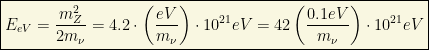
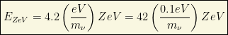

In fact, this mechanism based on “neutral resonances” is completely “universal”! Nothing (except some hidden symmetry or similar) can allow the production of (neutral) particles using this cosmic method. For instance, if this argument is true, beyond the Z-burst, we should be able to detect Higgs-dips (Higgs-bursts) or H-dips, since, similarely we could have

or more generally, with some (likely) “dark” particle, we should also expect that

In the H-dip case, taking the measured Higgs mass from the last LHC run (about 126GeV), we get


In the arbitrary “dark” or “weakly interacting” particle, we have (in general, with 


Therefore, cosmic ray neutrino spectroscopy is a very interesting subject yet to come! It can provide:
1st. Evidences for relic neutrinos we expect from the standard cosmological model.
2nd. Evidence for the Higgs boson in astrophysical scenarios from cosmological neutrinos. Now, we know that the Higgs field and the Higgs particle do exist, so it is natural to seek out this H-dips as well!
3rd. Evidence for the additional neutral weakly interacting (and/or “dark”) particles from “unexpected” dips at ZeV (1ZeV=1Zetta electron-volt) or even higher energies! Of course, this is the most interesting part from the viewpoint of new physics searches!
Neutrino telescopes and their associated Astronomy is just rising now! IceCube is its most prominent example…
Moreover, following one of the most interesting things in any research (expect the unexpected and try to explain it!) from the scientific viewpoint, I am quite sure the neutrino astronomy and its interplay with cosmic rays or this class of “neutrino spectroscopy” in the flux of cosmic rays open a very interesting window for the upcoming new physics. Are we ready for it? Maybe…After all, the neutrino mixing parameters are very different (“complementary”?) to the quark mixing parameters. You can observe it in this mass-flavor content plot:
 Neutrino oscillations are a purely quantum effect, and thus, they open a really interesting “new channel” in which we can observe the whole Universe. Yes, neutrinos are cool!!! The coolest particles in all over the world! We can not imagine yet what neutrino will show and teach us about the current, past and future of the cosmological evolution.

Remark: When I saw the Fermi line and the claim of the Dark Matter particle “evidence” at about 130 GeV, I wondered if it could be, indeed, a hint of a similar “resonant” process in gamma rays, something like

since the line “peaked” close to the known Higgs-like particle mass (
Final (geek) remark: I wonder if the Doctor Who fans remember that the reality bomb of Davros and the Daleks used “Z-neutrinos“!!! I presently do not know if the people who wrote those scripts and imagined the Z-neutrino were aware of the Z-bursts…Or not… LOL The Z-neutrino powered crucible was really interesting…

And the reality bomb concept was really scaring…

However, neutrinos are pretty weakly interacting particles, at least when they have low energy, so we should have not fear them. After all, their future applications will surprise us much more. I am quite sure of it!
See you in my next neutrinological post!
May the Z(X)-burst induced superGZK neutrinos be with you!
LOG#124. Basic Neutrinology(IX).
Posted: 2013/07/15 Filed under: Basic Neutrinology, Physmatics, The Standard Model: Basics | Tags: baryogenesis, baryon to entropy density ratio, baryon-antibaryon asymmetry, entropy ratio, hybrid inflation, inflationary phase, inflationary scenarios, inflaton, left-handed neutrinos, leptogenesis, lepton-antilepton asymmetry, LR models, neutrino masses, neutrinology, non-perturbative effects, Pati-Salam group, reheating, right-handed neutrinos, solar neutrino problem, sphaleron, superfields, SUSY Leave a commentIn supersymmetric LR models, inflation, baryogenesis (and/or leptogenesis) and neutrino oscillations can be closely related to each other. Baryosynthesis in GUTs is, in general, inconsistent with inflationary scenarios. The exponential expansion during the inflationary phase will wash out any baryon asymmetry generated previously by any GUT scale in your theory. One argument against this feature is the next idea: you can indeed generate the baryon or lepton asymmetry during the process of reheating at the end of inflation. This is a quite non-trivial mechanism. In this case, the physics of the “fundamental” scalar field that drives inflation, the so-called inflaton, would have to violate the CP symmetry, just as we know that weak interactions do! The challenge of any baryosynthesis model is to predict the observed asymmetry. It is generally written as a baryon to photon (in fact, a number of entropy) ratio. Tha baryon asymmetry is defined as

At present time, there is only matter and only a very tiny (if any) amount of antimatter, and then 


From BBN, we know that

and

This value allows to obtain the observed lepton asymmetry ratio with analogue reasoning.
By the other hand, it has been shown that the “hybrid inflation” scenarios can be successfully realized in certain SUSY LR models with gauge groups

after SUSY symmetry breaking. This group is sometimes called the Pati-Salam group. The inflaton sector of this model is formed by two complex scalar fields 


Remark: (Sphalerons). From the wikipedia entry we read that a sphaleron (Greek: σφαλερός “weak, dangerous”) is a static (time independent) solution to the electroweak field equations of the SM of particle physics, and it is involved in processes that violate baryon and lepton number.Such processes cannot be represented by Feynman graphs, and are therefore called non-perturbative effects in the electroweak theory (untested prediction right now). Geometrically, a sphaleron is simply a saddle point of the electroweak potential energy (in the infinite dimensional field space), much like the saddle point of the surface 

The resulting lepton asymmetry can be written as a function of a number of parameters among them the neutrino masses and the mixing angles, and finally, this result can be compared with the observational constraints above in baryon asymmetry. However, this topic is highly non-trivial. It is not trivial that solutions satisfying the constraints above and other physical requirements can be found with natural values of the model parameters. In particular, it is shown that the value of the neutrino masses and the neutrino mixing angles which predict sensible values for the baryon or lepton asymmetry turn out to be also consistent with values require to solve the solar neutrino problem we have mentioned in this thread.
LOG#123. Basic Neutrinology(VIII).
Posted: 2013/07/15 Filed under: Basic Neutrinology, Physmatics, The Standard Model: Basics | Tags: CDM, CMB, CNB, cold dark matter, cosmic neutrino background, cosmological constant, critical density, HDM, hot dark matter, matter density, neutrino astronomy, neutrino comoslogy, neutrino decoupling, neutrino mass bounds from cosmology, neutrinology, number of effective neutrino species, PLANCK, total matter density, Tremaine-Gunn limit, WMAP Leave a commentThere are some indirect constraints/bounds on neutrino masses provided by Cosmology. The most important is the one coming from the demand that the energy density of the neutrinos should not be too high, otherwise the Universe would collapse and it does not happen, apparently…
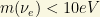
Firstly, stable neutrinos with low masses (about 

and where the total mass is defined to be the quantity

Here, the number of degrees of freedom 

From this, we can derive the relationship of the cosmic relic neutrino background (neutrinos coming from the Big Bang radiation when they lost the thermal equilibrium with photons!) or
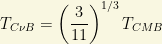
From the CMB radiation measurements we can obtain the value
for a perfect Planck blackbody spectrum with temperature

This CMB temperature implies that the

Remark: if you do change the number of neutrino degrees of freedom you also change the temperature of the
Moreover, the neutrino density 

and where the critical density is about

When neutrinos “decouple” from the primordial plasma and they loose the thermal equilibrium, we have 
with 
There is another useful requirement for the neutrino density in Cosmology. It comes from the requirements of the BBN (Big Bang Nucleosynthesis). I talked about this in my Cosmology thread. Galactic structure and large scale observations also increase evidence that the matter density is:

These values are obtained through the use of the luminosity-density relations, galactic rotation curves and the observation of large scale flows. Here, the 


are rather well known. The photon density is

The deuterium abundance can be extracted from the BBN predictions and compared with the deuterium abundances in the stellar medium (i.e. at stars!). It shows that:

The HDM component is formed by relativistic long-lived particles with masses less than about 
The simulations of structure formation made with (super)computers fit the observations ONLY when one has about 20% of HDM plus 80% of CDM. A stunning surprise certainly! Some of the best fits correspond to neutrinos with a total mass about 4.7eV, well above the current limit of neutrino mass bounds. We can evade this apparent contradiction if we suppose that there are some sterile neutrinos out there. However, the last cosmological data by PLANCK have decreased the enthusiasm by this alternative. The apparent conflict between theoretical cosmology and observational cosmology can be caused by both unprecise measurements or our misunderstanding of fundamental particle physics. Anyway observations of distant objects (with high redshift) favor a large cosmological constant instead of Hot Dark Matter hypothesis. Therefore, we are forced to conclude that the HDM of 


Mass limits, in this case lower limits, for heavy or superheavy neutrinos (
There is another interesting limit to the density of neutrinos (or weakly interacting dark matter in general) that comes from the amount of accumulated “density” in the halos of astronomical objects. This is called the Tremaine-Gunn limit. Up to numerical prefactors, and with the simplest case where the halo is a singular isothermal sphere with 

Imposing the phase space bound at radius r then gives the lower bound

This bound yields 
Remark: The singular isothermal sphere is probably a good model where the rotation curve produced by the dark matter halo is flat, but certainly breaks down at small radius. Because the neutrino mass bound is stronger for smaller 
The abundance of additional weakly interacting light particles, such as a light sterile neutrino 


PLANCK data suggest indeed that 
LOG#122. Basic Neutrinology(VII).
Posted: 2013/07/15 Filed under: Basic Neutrinology, Physmatics, The Standard Model: Basics | Tags: anomalies, anomalous terms, beyond SM, BSM, Cabibble angle, family symmetry, Froggatt, gauge anomalies, mass hierarchy, neutrino mass from family symmetry, neutrinology, New Physics, particle physics, quark and lepton complementarity, seesaw mechanism, spontaneous symmetry breaking, SSB, U(1) hidden symmetry, vev Leave a commentThe observed mass and mixing both in the neutrino and quark cases could be evidence for some interfamily hierarchy hinting that the lepton and quark sectors were, indeed, a result of the existence of a new quantum number related to “family”. We could name this family symmetry as 

A simple model with one family dependent anomalous U(1) beyond the SM was first proposed long ago to produce the given Yukawa coupling and their hierarchies, and the anomalies could be canceled by the Green-Schwarz mechanism which as by-product is able to fix the Weinberg angle as well. Several developments include the models inspired by the 


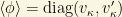
The 3 symmetries and their fields 


and where 


and where 


From these matrices, the associated seesaw mechanism gives the formula for light neutrinos:

The neutrino mass mixing matrix depends only on the charges we assign to the LH neutrinos due to cancelation of RH neutrino charges and the seesaw mechanism. There is freedom in the assignment of the charges 


and where 


LOG#121. Basic Neutrinology(VI).
Posted: 2013/07/15 Filed under: Basic Neutrinology, Physmatics, The Standard Model: Basics | Tags: 3-brane, bulk, bulk mode, bulk state, extra dimensions, extra space-like dimension, KK resonance, KK state, KK tower, left-handed neutrino, model building, neutrino mass matrix from extra dimensions, neutrinology, non-factorirable metric, Planck scale, Randall-Sundrum model, renormalizability, right-handed neutrino, SM brane, sterile neutrino, submicrometer extra dimension, submillimeter extra dimension Leave a commentModels where the space-time is not 3+1 dimensional but higher dimensional (generally D=d+1=4+n dimensional, where n is the number of spacelike extra dimensions) are popular since the beginnings of the 20th century.
The fundamental scale of gravity need not to be the 4D “effective” Planck scale 


Here, 


According to the SM and the standard gravity framework (General Relativity), every group charged particle is localized on a 3-dimensional hypersurface that we could call “brane” (or SM brane). This brane is embedded in “the bulk” of the higher dimensional Universe (with 
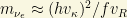
The small coupling constant derived from the Planck mass above can also be used in order to explain the smallness of the neutrino masses! The left-handed neutrino 


Here, 

The right-handed neutrino 


and the

with

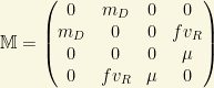
Are you afraid of “infinite” neutrino flavors? The resulting neutrino mass matrix M is “an infinite array” with structure:
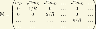
The eigenvalues of the matrix 


The main issues that extra dimension models of neutrino masses do have is related to the question of the renormalizability of their interactions. With an infinite number of KK states and/or large extra dimensions, extreme care have to be taken in order to not spoil the SM renormalizability and, at some point, it implies that the KK tower must be truncated at some level. There is no general principle or symmetry that explain this cut-off to my knowledge.
May the neutrinos and the extra dimensions be with you!
See you in my next neutrinological post!
LOG#120. Basic Neutrinology(V).
Posted: 2013/07/15 Filed under: Basic Neutrinology, Physmatics, The Standard Model: Basics | Tags: bino, dark matter, Dirac mass term, E(6) group, exceptional group GUT, gauginos, GUT, GUT scale, Higgsino, LR models, LSP, Majorana mass term, MSSM, neutralino, neutrino masses, neutrino mixing, proton decay, proton lifetime, R-parity, R-parity violations, seesaw, sfermion, singlets, sneutrino, soft SUSY breaking terms, string inspired models, superparticle, superpartner, superpotential, SUSY models of neutrino masses, vev, WIMPs, wino, Yukawa coupling, Zinos Leave a commentSupersymmetry (SUSY) is one of the most discussed ideas in theoretical physics. I am not discussed its details here (yet, in this blog). However, in this thread, some general features are worth to be told about it. SUSY model generally include a symmetry called R-parity, and its breaking provide an interesting example of how we can generate neutrino masses WITHOUT using a right-handed neutrino at all. The price is simple: we have to add new particles and then we enlarge the Higgs sector. Of course, from a pure phenomenological point, the issue is to discover SUSY! On the theoretical aside, we can discuss any idea that experiments do not exclude. Today, after the last LHC run at 8TeV, we have not found SUSY particles, so the lower bounds of supersymmetric particles have been increased. Which path will Nature follow? SUSY, LR models -via GUTs or some preonic substructure, or something we can not even imagine right now? Only experiment will decide in the end…
In fact, in a generic SUSY model, dut to the Higgs and lepton doublet superfields, we have the same 

(1)

A less radical solution is to allow for the existence in the superpotential of a bilinear term with structure 


(2)

and where the matrix 


I should explain a little more the supersymmetric terminology. The neutralino is a hypothetical particle predicted by supersymmetry. There are some neutralinos that are fermions and are electrically neutral, the lightest of which is typically stable. They can be seen as mixtures between binos and winos (the sparticles associated to the b quark and the W boson) and they are generally Majorana particles. Because these particles only interact with the weak vector bosons, they are not directly produced at hadron colliders in copious numbers. They primarily appear as particles in cascade decays of heavier particles (decays that happen in multiple steps) usually originating from colored supersymmetric particles such as squarks or gluinos. In R-parity conserving models, the lightest neutralino is stable and all supersymmetric cascade-decays end up decaying into this particle which leaves the detector unseen and its existence can only be inferred by looking for unbalanced momentum (missing transverse energy) in a detector. As a heavy, stable particle, the lightest neutralino is an excellent candidate to comprise the universe’s cold dark matter. In many models the lightest neutralino can be produced thermally in the hot early Universe and leave approximately the right relic abundance to account for the observed dark matter. A lightest neutralino of roughly 
Neutralino dark matter could be observed experimentally in nature either indirectly or directly. In the former case, gamma ray and neutrino telescopes look for evidence of neutralino annihilation in regions of high dark matter density such as the galactic or solar centre. In the latter case, special purpose experiments such as the (now running) Cryogenic Dark Matter Search (CDMS) seek to detect the rare impacts of WIMPs in terrestrial detectors. These experiments have begun to probe interesting supersymmetric parameter space, excluding some models for neutralino dark matter, and upgraded experiments with greater sensitivity are under development.
If we return to the matrix (2) above, we observe that when we diagonalize it, a “seesaw”-like mechanism is again at mork. There, the role of 


where 


(3)

We can study now the elementary properties of neutrinos in some elementary superstring inspired models. In some of these models, the effective theory implies a supersymmetric (exceptional group) 


(4)

and where the 
1st. R-parity violation.
2nd. R-parity conservation and a “mixing” with the singlet.
In both cases, the sneutrinos, superpartners of 


In the second case, the field 
Final remark: mass matrices, as we have studied here, have been proposed without embedding in a supersymmetric or any other deeper theoretical frameworks. In that case, small tree level neutrino masses can be obtained without the use of large scales. That is, the structure of the neutrino mass matrix is quite “model independent” (as the one in the CKM quark mixing) if we “measure it”. Models reducing to the neutrino or quark mass mixing matrices can be obtained with the use of large energy scales OR adding new (likely “dark”) particle species to the SM (not necessarily at very high energy scales!).
LOG#119. Basic Neutrinology(IV).
Posted: 2013/07/14 Filed under: Basic Neutrinology, Physmatics, The Standard Model: Basics | Tags: GUT, LR models, neutrinology, seesaw mechanism, SO(10) unification, SUSY unification Leave a commentA very natural way to generate the known neutrino masses is to minimally extend the SM including additional 2-spinors as RH neutrinos and at the same time extend the non-QCD electroweak SM gauge symmetry group to something like this:

The resulting model, initially proposed by Pati and Salam (Phys. Rev. D.10. 275) in 1973-1974. Mohapatra and Pati reviewed it in 1975, here Phys. Rev. D. 11. 2558. It is also reviewed in Unification and Supersymmetry: the frontiers of Quark-Lepton Physics. Springer-Verlag. N.Y.1986. This class of models were first proposed with the goal of seeking a spontaneous origin for parity (P) violations in weak interactions. CP and P are conserved at large energies but at low energies, however, the group 


and where

If we choose the alternative 
The quarks 


The breaking of the gauge symmetry is implemented by multiplets of LR symmetric Higgs fields. The concrete selection of these multiplets is NOT unique. It has been shown that in order to understand the smallness of the neutrino masses, it is convenient to choose respectively one doublet and two triplets in the following way:


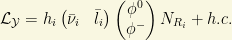
The Yukawa couplings of these Higgs fields with the quarks and leptons are give by the lagrangian term


The gauge symmetry breaking in LR models happens in two steps:
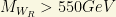
1st. The 


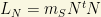
Furthermore, as consequence of the f-term in the lagrangian, above this stage of symmetry breaking also leads to a mass term for the right-handed neutrinos with order about 
2nd. As we break the SM symmetry by turning on the vev’s for the scalar fields


We give masses to the 


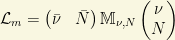
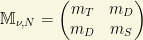
In the neutrino sector, the above Yukawa couplings after 


corresponding to the lighter and more massive neutrino states after the diagonalization procedure. In fact, the seesaw mechanism implies the eigenvalue
for the lowest mass, and the eigenvalue

for the (super)massive neutrino state. Several variants of the basic LR models include the option of having Dirac neutrinos at the expense of enlarging the particle content. The introduction of two new single fermions and a new set of carefully chosen Higgs bosons, allows us to write the 
This matrix leads to two different Dirac neutrinos, one heavy with mass 


Left-Right symmetric(LR) models can be embedded in grand unification groups. The simplest GUT model that leads by successive stages of symmetry breaking to LR symmetric models at low energies is 
LOG#118. Basic Neutrinology(III).
Posted: 2013/07/13 Filed under: Basic Neutrinology, Physmatics, The Standard Model: Basics | Tags: Dirac mass term, GUT baryon-lepton mass models, GUTs, LR models, magnetic dipole moments, Majorana fermion, Majorana mass term, mass terms, neutrinology, New Physics, pseudo-Dirac fermion, seesaw, seesaw limit, seesaw types, singlet mass term, SO(10), triplet mass term Leave a comment

Mass terms

Phenomenologically, lagrangian mass terms can be understood as terms describing “transitions” between right (R) and left (L) handed states in the electroweak sector. For a given minimal, Lorentz invariant set of 4 fields (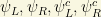

In terms of a “new” Majorana (real) field with 


and then, the massive lagrangian becomes
where the neutrino mass matrix is defined to be
We can diagonalize this mass matrix and then we will find the physical particle content! It is given (in general) by two Majorana mass eigenstates: the inclusion of the Majorana mass splits the 4 degenerate states of the Dirac field into two non-degenerate Majorana pairs. If we assume that the states 


The seesaw

When we diagonalize the above neutrino mass matrix, we can analyze different “limit” cases. In the case of a purely Dirac mass term, i.e., whenver 


In the general case, pure Majorana mass transition terms (

When every mass term is allowed, there is an interesting case commonly referred as “the seesaw” limit. In this limit, taking the triplet mass to be zero and the singlet mass to be “huge” or “superheavy”, we deduce that


In this seesaw limit, the neutrino mass matrix can be diagonalized and it provides two eigenvalues:
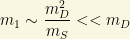

Thus, the seesaw mechanism provide a way in which we obtain two VERY different mass eigenstates, i.e., two single particle states separated by a huge mass hierarchy! There is one (super)heavy neutrino (generally speaking, it corresponds to the right-handed neutrino) and a much lighter neutrino state, one that can be made relatively much lighter than a normal Dirac fermion mass. One fo the neutrino mass is “suppressed” and balanced up (hence the name “seesaw”) by the (super)heavy species. The seesaw mechanism is a “natural” way of generating two different (often VERY separated) mass scales!
The theory of the seesaw mechanism is very rich. I will not discuss its full potential here. There are 3 main types of seesaw mechanisms (generally named as type I, type II and type III) and some other less frequent variants and subvariants…It is an advanced topic for a whole future thread! 😉 However, I will draw you the 3 main Feynman graphs involved in these 3 main types of seesaw mechanisms:

GUTs and neutrino mass models

Any fully satisfactory model that generates neutrino masses must contain a natural mechanism which allows us to explain their samll value, relative to that of their charged partners. Given the latest experimental hints and results, it would also be possible that it will include any comprehensive explanation for light sterile neutrinos and large, nearl maximal, mixing. This last idea is due to some “anomalies” coming from some neutrino experiments (specially those coming from reactors and the celebrated LSND experiment).
Different models can be distinguished according to the new particle content and spectrum, or according to the energy scale hierarchy they produce. With an extended particle content, different options open: if we want to brak the lepton number ant to generate neutrino masses without introducing new (unobserved) fermions in the SM, we must do it by adding to the SM Higgs sector fields carrying lepton numbers. Thus, one can arrange them to break the lepton number explicitly or spontaneously through interactions with these fields. If you want, this is another reason why the Higgs field matters: it allows to introduce fields carrying lepton numbers without adding any extra fermion field! Likely, the most straightforward approach to generate neutrino masses is to introduce for each neutrino an additional weak neutral single (that can be identified with the right-handed neutrino we can not observed due to be “very massive” and/or uncharged under the SM gauge group). This last fact strongly favors seesaw-like models!
For instance, the above features happen in the framework of LR (Left-Right) symmetric models in Grand Unified Theories (GUTs). There, the origin of the SM parity violation (explicit in the electroweak and weak sectors) is due to the spontaneous symmetry breaking of a baryon-lepton symmetry, and it yields a 

If we use the energy scale as a guide where the new physics have relevant effects, unification (e.g., think about the previous SO(10) example) and the weak scale approach (radiative models and their effective theories) are usually distinguished and preferred form a pure QFT approach.
Despite the fact that the explanation of the known neutrino anomalies (the solar neutrino problem the first, but also the atmospheric neutrino flux and the reactor anomalies/neutrino beam anomalies) do not need or require the existence of an additional extra light/heavy sterile neutrino, some authors claim that they could exist after all. If every Marojana mass term is “small enough”, then active neutrinos can oscillate or mix into sterile (likely right-handed) fields/states. Light sterile neutrinos can appear in particularly special see-saw mechanisms if additional assumptions are considered (there, some models called “singular seesaw” models do exist as well). with some inevitable amount of “fine tuning”. The alternative to “fine tuning” would be seesaw-like suppression for sterile neutrinos involving new unknown (likely ultraweak or “dark”) interactions, i.e., family symmetries resulting in substantial field additions to the SM (some string theory models also suggest this possibility).
There is also weak scale models, i.e., radiative generated mass models where the neutrino masses are zero at tree level and they constitute a very different type of models: they explain the smallness of the neutrino masses a priori for both active and sterile neutrinos. Loop corrections induce neutrino mass terms in these models. Thus, different mass scales are generated naturally by the different number of loops involved in the generation of each term. The actual implementation requires, however, the ad hoc (a posteriori) introduction of new Higgs particles with non-standard electroweak quantum numbers and lepton number violating couplings. This is the price we pay in an alternative approach.
The origin of the different Dirac and Majorana mass terms 

Here, 


In the case of the Majorana mass term, the 

is allowed by the SM gauge group. However, it would bot be consistent in general with unified symmetries or general GUTs. That is, a full SO(10), for instance, and some complicated mechanisms should be used to describe and explain the presence of this term. The 

When the 


1) An elementary Higgs triplet.
2) An effective operator involving two Higgs doublets arranged to transform as a triplet.
In both cases, we can induce non-renormalizable interactions. In case 1), an elementary triplet 


Final remarks: If 


Neutrinos and magnetic dipole moments
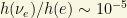
The magnetic dipole moment is another probe of possible new interactions and physics beyond the Standard Model. Majorana neutrinos have identically zero magnetic and electric dipole moments. Flavor transition magnetic moments are allowed however in general for both Dirac and Majorana neutrinos! Limits obtained from laboratory experiments (LEX) are of the order of a constant times 


The proportionality of 

These values are still too small to have odds of being measurable in current experiments or having practical astrophysical or cosmological consequences we could detect now. However, these magnetic dipole moments are important features of BSM models, so it is important to study them.
Magnetic moment interactions arise in ANY renormalizable gauge theory only as finite radiative corrections. The diagrams which generate a magnetic moment will also contribute to the neutrino mass once the external photon line is removed.In the absence of additional symmetries, a large magnetic moment is incompatible with a small neutrino mass. The way out to this NO-GO theorem suggested by Voloshin consists in defining a 

What do you think? Some novel idea? Here you are a decision tree map (LOL):
 However, we are far, far away to understand the neutrino hidden higher secrets! Here you are a basic “road map” towards superbeams and neutrino factories, yet an intermediate step before the mythical muon collider (yes, USA likely WANTS that muon collider, :P)…
 May the neutrinos be with you!
PS: See you in my next neutrinology blog post!


You must be logged in to post a comment.