LOG#080. A Bug-Rivet “paradox”.

Posted: 2013/04/07 | Author: amarashiki | Filed under: Physmatics, Relativity | Tags: bug-rivet paradox, paradox, Relativity, special relativity | 1 Comment

Imagine that an idealised bug of negligible dimensions is hiding at the end of a hole of length L. A rivet has a shaft length of $a<L$ .

Clearly the bug is “safe” when the rivet head is flush to the (very resiliente) surface. The problem arises as follows. Consider what happens when the rivet slams into the surface at a speed of $v=\beta c$ , where c is the speed of light and $0<\beta<1$ . One of the essences of the special theory of relativity is that objects moving relative to our frame of reference are shortened in the direction of motion by a factor $\gamma^{-1}=\sqrt{1-\beta^2}$ , where $\gamma$ is generally called the Lorentz dilation factor, as readers of this blog already know. However, from the point of view (frame of reference) of the bug, the rivet shaft is even shorter and therefore the bug should continue to be safe, and thus fast the rivet is moving.

Apparently, we have:

$a_{app}=\dfrac{a}{\gamma}=a\sqrt{1-\beta^2}$

Remark: this idea assumes that both objects are ideally rigid! We will return to this “fact” later.

From the frame of reference of the rivet, the rivet is stationary and unchanged, but the hole is moving fast and is shortened by the Lorentz contraction to

$L_{app}=\dfrac{L}{\gamma}=L\sqrt{1-\beta^2}$

If the approach speed is fast enough, so that $L_{app}<a$ , then the end of the hole slams into the tip of the rivet before the surface
can reach the head of the rivet. The bug is squashed! This is the “paradox”: is the bug squashed or not?

There are many good sources for this paradox (a relative of the pole-barn paradox), such as:
1)http://en.wikipedia.org/wiki/Wikipedia:Reference_desk/Archives/Science/2006_October_19#Bug_Rivet_Paradox

2) A nice animation can be found here http://math.ucr.edu/~jdp/Relativity/Bug_Rivet.html

In this blog post we are going to solve this “paradox” in the framework of special relativity.

SOLUTION

One of the consequences of special relativity is that two events that are simultaneous in one frame of reference are no longer simultaneous in other frames of reference. Perfectly rigid objects are impossible.

In the frame of reference of the bug, the entire rivet cannot come to a complete stop all at the same instant. Information
cannot travel faster than the speed of light. It takes time for knowledge that the rivet head has slammed into the surface to
travel down the shaft of the rivet. Until each part of the shaft receives the information that the rivet head has stopped, that part keeps going at speed $v=\beta c$ . The information proceeds down the shaft at speed c while the tip continues to move at speed $v=\beta c$ .

The tip cannot stop until a time

$T_1=\dfrac{\dfrac{a}{\gamma}}{c-\beta c}=\dfrac{a}{\gamma c (1-\beta)}$

after the head has stopped. During that time the tip travels a distance $D_1=vT_1$ . The bug will be squashed if

$vT_1>L-\dfrac{a}{\gamma}$

This implies that

$\dfrac{\beta c a}{\gamma c (1-\beta)}>L-\dfrac{a}{\gamma}\leftrightarrow \dfrac{a}{\gamma}\left(\dfrac{\beta}{1-\beta}+1\right) >L\leftrightarrow \dfrac{a}{\gamma}\left(\dfrac{\beta+1-\beta}{1-\beta}\right) >L$

From $\gamma^{-1}=\sqrt{1-\beta^2}$ we can calculate that

$\dfrac{1}{\gamma (1-\beta)}=\dfrac{\sqrt{1-\beta^2}}{1-\beta}=\dfrac{\sqrt{(1+\beta)(1-\beta)}}{1-\beta}=\sqrt{\dfrac{1+\beta}{1-\beta}}$

The bug will be squashed if the following condition holds

$a\sqrt{\dfrac{1+\beta}{1-\beta}}>L\leftrightarrow \dfrac{a}{L}>\sqrt{\dfrac{1-\beta}{1+\beta}}\leftrightarrow \left(\dfrac{a}{L}\right)^2> \dfrac{1-\beta}{1+\beta}$

or equivalently, after some algebraic manipulations, the bug will be squashed if:

$\beta>\dfrac{1-\left(\dfrac{a}{L}\right)^2}{1+\left(\dfrac{a}{L}\right)^2}$

Conclusion (in bug’s reference frame): the bug will be definitively squashed when $v_{min}=\beta_{min}c$ such as

$\boxed{\beta_{min}=\dfrac{1-\left(\dfrac{a}{L}\right)^2}{1+\left(\dfrac{a}{L}\right)^2}}$

Check: It can be verified that the limits $\displaystyle{\lim_{a\rightarrow 0^+}\beta_{min}=1^{-}}$ and $\displaystyle{\lim_{a\rightarrow L^-}\beta_{min}=0^{+}}$ are valid and physically meaningful.

Note that the impact of the rivet head always happens before the bug is squashed.

In the frame of reference of the rivet, the bug is definitively squashed whenever $\dfrac{L}{\gamma}<a$ .

Then,

$L\sqrt{1-\beta^2}<a\leftrightarrow 1-\beta^2<\left(\dfrac{a}{L}\right)^2$

or equivalently

$\beta>\sqrt{1-\left(\dfrac{a}{L}\right)^2}$

$\beta>\beta_{min2}$ where $\boxed{\beta_{min2}=\sqrt{1-\left(\dfrac{a}{L}\right)^2}}$

The bug is squashed before the impact of the surface on the rivet head. This last equation (and thus $\beta_{min2}$ ) is a velocity higher than $\beta_{min}$ .

Conclusion (in rivet’s reference frame): The entire surface cannot come to an abrupt stop at the same instant. It takes time for the information about the impact of the rivet tip on the end of the hole to reach the surface that is rushing towards the rivet head. Let us now examine the case where the speed is not high enough for the Lorentz-contracted hole to be shorter than the rivet shaft in the frame of reference of the rivet. Now the observers agree that the impact of the rivet head happens first. When the surface slams into contact with the head of the rivet, it takes time for information about that impact to travel down to the end of the hole. During this time the hole continues to move towards the tip of the rivet.

The time it takes for the propagating information to reach the tip of the stationary rivet is

$T_2=\dfrac{a}{c}$

during which time the bug moves a distance $D_2=vT_2=\dfrac{\beta c a}{c}=\beta a$

In the rivet’s reference frame, therefore, The bug is squashed if the following condition holds

$vT_2>\dfrac{L}{\gamma}-a\leftrightarrow \beta a>\dfrac{L}{\gamma}-a\leftrightarrow (1+\beta)a>\dfrac{L}{\gamma}\leftrightarrow \dfrac{a}{L}>\dfrac{1}{1+\beta}\sqrt{1-\beta^2}$

and then

$\dfrac{\sqrt{(1+\beta)(1-\beta)}}{1+\beta}<\dfrac{a}{L}\leftrightarrow \sqrt{\dfrac{1-\beta}{1+\beta}}<\dfrac{a}{L}$

and from this equation, we get same minimum speed that guarantees the squashing of the bug as was the case in the frame of reference of the bug! That is:

$\boxed{\beta_{min}=\dfrac{1-\left(\dfrac{a}{L}\right)^2}{1+\left(\dfrac{a}{L}\right)^2}}$

Note that observers travelling with each of the two frames of reference (bug and rivet) agree that the bug is squashed IF $\beta>\beta_{min}$ , and that resolves the “paradox”. They also agree that the impact of rivet head on surface happens before the bug is squashed, provided that the following condition is satisfied:

$\beta_{min}<\beta<\beta_{min2}$

i.e., they agree if the impact of rivet head on surface happens before the bug is squashed

$\boxed{\dfrac{1-\left(\dfrac{a}{L}\right)^2}{1+\left(\dfrac{a}{L}\right)^2}<\beta<\sqrt{1-\left(\dfrac{a}{L}\right)^2}}$

Otherwise, they disagree on which event happens first. For instance, if

$\beta>\beta_{min2}=\sqrt{1-\left(\dfrac{a}{L}\right)^2}$

For speeds this high, the observer in the bug’s frame of reference still deduces that the rivet-head impact happens first, but the other observer deduces that the bug is squashed first. This is consistent with the relativity of simultaneity! At the critical speed, when $\beta=\beta_c=\beta_{min2}$ the two events are simultaneous in the frame of the rivet, (the river fits perfectly in the shortened hole), but they are not simultaneous in the other frame of reference.

See you in the next blog post!

LOG#075. Batmobile “paradox”.

Posted: 2013/02/11 | Author: amarashiki | Filed under: Physmatics, Relativity | Tags: fake paradox, paradox, Relativity, simultaneity, special relativity | Leave a comment

The Batmobile “fake paradox” helps us to understand Special Relativity a little bit. This problem consists in the next experiment:

There are two observers. Alfred, the external observer, and Batman moving with his Batmobile.

Now, we will suppose that the Batmobile is moving at a very fast constant speed with respect to the garage. Let us suppose that $v=0.866c=\dfrac{\sqrt{3}}{2}c$ . Then, we have the following situation from the external observer:

However, with respect to the Batmobile reference frame, we have:

The question is. Who is right? Alfred or Batman? The surprinsig answer from Special Relativity is that Both are correct. Alfred and Batman are right! Let’s see why it is true. For Alfred, there is a time during which the Batmobile is completely inside the garage with both doors closed:

By the other hand, for Batman, the front and rear doors are not closed simultaneously! So there is never a time during which the Batmobile is completely inside the garage with both doors closed.

So, there is no paradox at all, if you are aware about the notion of simultaneity and its relativity!

LOG#070. Natural Units.

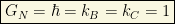
Posted: 2013/01/30 | Author: amarashiki | Filed under: Classical and Quantum Fields, Cosmology, Gravitational theories, Physmatics, Quantum Gravity, Relativity, The Standard Model: Basics, Units, natural units and metrology | Tags: amount of substance, atomic units, Boltzmann constant, coulomb constant, electric charge, electric current, electric permitivy of vacuum, electromagnetism, ELKO field, Fritzsch-Xing plot, geometrized units, gravitation, gravitational constant, hep units, luminous intensity, mass, mass dimension of fields, MKSA units, mole, natural units, Okun cube, Planck constant, planck units, QCD units, Quantum Gravity, schrödinger units, space, spacetime, speed of light, stoney units, time, TOE, vacuum | 1 Comment

Happy New Year 2013 to everyone and everywhere!

Let me apologize, first of all, by my absence… I have been busy, trying to find my path and way in my field, and I am busy yet, but finally I could not resist without a new blog boost… After all, you should know the fact I have enough materials to write many new things.

So, what’s next? I will dedicate some blog posts to discuss a nice topic I began before, talking about a classic paper on the subject here:

https://thespectrumofriemannium.wordpress.com/2012/11/18/log054-barrow-units/

The topic is going to be pretty simple: natural units in Physics.

First of all, let me point out that the election of any system of units is, a priori, totally conventional. You are free to choose any kind of units for physical magnitudes. Of course, that is not very clever if you have to report data, so everyone can realize what you do and report. Scientists have some definitions and popular systems of units that make the process pretty simpler than in the daily life. Then, we need some general conventions about “units”. Indeed, the traditional wisdom is to use the international system of units, or S (Iabbreviated SI from French language: Le Système international d’unités). There, you can find seven fundamental magnitudes and seven fundamental (or “natural”) units:

1) Space: $\left[ L\right]=\mbox{meter}=m$

2) Time: $\left[ T\right]=\mbox{second}=s$

3) Mass: $\left[ M\right]=\mbox{kilogram}=kg$

4) Temperature: $\left[ t\right]=\mbox{Kelvin degree}= K$

5) Electric intensity: $\left[ I\right]=\mbox{ampere}=A$

6) Luminous intensity: $\left[ I_L\right]=\mbox{candela}=cd$

7) Amount of substance: $\left[ n\right]=\mbox{mole}=mol(e)$

The dependence between these 7 great units and even their definitions can be found here http://en.wikipedia.org/wiki/International_System_of_Units and references therein. I can not resist to show you the beautiful graph of the 7 wonderful units that this wikipedia article shows you about their “interdependence”:

In Physics, when you build a radical new theory, generally it has the power to introduce a relevant scale or system of units. Specially, the Special Theory of Relativity, and the Quantum Mechanics are such theories. General Relativity and Statistical Physics (Statistical Mechanics) have also intrinsic “universal constants”, or, likely, to be more precise, they allow the introduction of some “more convenient” system of units than those you have ever heard ( metric system, SI, MKS, cgs, …). When I spoke about Barrow units (see previous comment above) in this blog, we realized that dimensionality (both mathematical and “physical”), and fundamental theories are bound to the election of some “simpler” units. Those “simpler” units are what we usually call “natural units”. I am not a big fan of such terminology. It is confusing a little bit. Maybe, it would be more interesting and appropiate to call them “addapted X units” or “scaled X units”, where X denotes “relativistic, quantum,…”. Anyway, the name “natural” is popular and it is likely impossible to change the habits.

In fact, we have to distinguish several “kinds” of natural units. First of all, let me list “fundamental and universal” constants in different theories accepted at current time:

1. Boltzmann constant: $k_B$ .

Essential in Statistical Mechanics, both classical and quantum. It measures “entropy”/”information”. The fundamental equation is:

$\boxed{S=k_B\ln \Omega}$

It provides a link between the microphysics and the macrophysics ( it is the code behind the equation above). It can be understood somehow as a measure of the “energetic content” of an individual particle or state at a given temperature. Common values for this constant are:

$k_B=1.3806488(13)\times 10^{-23}J/K = 8.6173324(78)\times 10^{-5}eV/K$

$k_B=1.3806488(13)\times 10^{-16}erg/K$

Statistical Physics states that there is a minimum unit of entropy or a minimal value of energy at any given temperature. Physical dimensions of this constant are thus entropy, or since $E=TS$ , $\left[ k_B\right] =E/t=J/K$ , where t denotes here dimension of temperature.

2. Speed of light. $c$ .

From classical electromagnetism:

$\boxed{c^2=\dfrac{1}{\sqrt{\varepsilon_0\mu_0}}}$

The speed of light, according to the postulates of special relativity, is a universal constant. It is frame INDEPENDENT. This fact is at the root of many of the surprising results of special relativity, and it took time to be understood. Moreover, it also connects space and time in a powerful unified formalism, so space and time merge into spacetime, as we do know and we have studied long ago in this blog. The spacetime interval in a D=3+1 dimensional space and two arbitrary events reads:

$\Delta s^2=\Delta x^2+\Delta y^2+\Delta z^2-c^2\Delta t^2$

In fact, you can observe that “c” is the conversion factor between time-like and space-like coordinates. How big the speed of light is? Well, it is a relatively large number from our common and ordinary perception. It is exactly:

$\boxed{c=299,792,458m/s}$

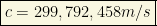
although you often take it as $c\approx 3\cdot 10^{8}m/s=3\cdot 10^{10}cm/s$ . However, it is the speed of electromagnetic waves in vacuum, no matter where you are in this Universe/Polyverse. At least, experiments are consistent with such an statement. Moreover, it shows that $c$ is also the conversion factor between energy and momentum, since

$\mathbf{P}^2c^2-E^2=-m^2c^4$

and $c^2$ is the conversion factor between rest mass and pure energy, because, as everybody knows, $E=mc^2$ ! According to the special theory of relativity, normal matter can never exceed the speed of light. Therefore, the speed of light is the maximum velocity in Nature, at least if specially relativity holds. Physical dimensions of c are $\left[c\right]=LT^{-1}$ , where L denotes length dimension and T denotes time dimension (please, don’t confuse it with temperature despite the capital same letter for both symbols).

3. Planck’s constant. $h$ or generally rationalized $\hbar=h/2\pi$ .

Planck’s constant (or its rationalized version), is the fundamental universal constant in Quantum Physics (Quantum Mechanics, Quantum Field Theory). It gives

$\boxed{E=h\nu=\hbar \omega}$

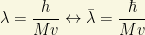
Indeed, quanta are the minimal units of energy. That is, you can not divide further a quantum of light, since it is indivisible by definition! Furthermore, the de Broglie relationship relates momentum and wavelength for any particle, and it emerges from the combination of special relativity and the quantum hypothesis:

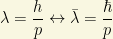
$\lambda=\dfrac{h}{p}\leftrightarrow \bar{\lambda}=\dfrac{\hbar}{p}$

In the case of massive particles, it yields

$\lambda=\dfrac{h}{Mv}\leftrightarrow \bar{\lambda}=\dfrac{\hbar}{Mv}$

In the case of massless particles (photons, gluons, gravitons,…)

$\lambda=\dfrac{hc}{E}$ or $\bar{\lambda}=\dfrac{\hbar c}{E}$

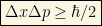
Planck’s constant also appears to be essential to the uncertainty principle of Heisenberg:

$\boxed{\Delta x \Delta p\geq \hbar/2}$

$\boxed{\Delta E \Delta t\geq \hbar/2}$

$\boxed{\Delta A\Delta B\geq \hbar/2}$

Some particularly important values of this constant are:

$h=6.62606957(29)\times 10^{-34} J\cdot s$
$h=4.135667516(91)\times 10^{-15}eV\cdot s$
$h=6.62606957(29)\times 10^{-27} erg\cdot s$
$\hbar =1.054571726(47)\times 10^{-34} J\cdot s$
$\hbar =6.58211928(15)\times 10^{-16} eV\cdot s$
$\hbar= 1.054571726(47)\times 10^{-27}erg\cdot s$

It is also useful to know that
$hc=1.98644568\times 10^{-25}J\cdot m$
$hc=1.23984193 eV\cdot \mu m$

$\hbar c=0.1591549hc$ or $\hbar c=197.327 eV\cdot nm$

Planck constant has dimension of $\mbox{Energy}\times \mbox{Time}=\mbox{position}\times \mbox{momentum}=ML^2T^{-1}$ . Physical dimensions of this constant coincide also with angular momentum (spin), i.e., with $L=mvr$ .

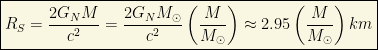
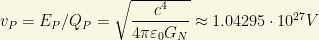
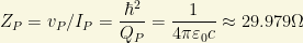
4. Gravitational constant. $G_N$ .

Apparently, it is not like the others but it can also define some particular scale when combined with Special Relativity. Without entering into further details (since I have not discussed General Relativity yet in this blog), we can calculate the escape velocity of a body moving at the speed of light

$\dfrac{1}{2}mv^2-G_N\dfrac{Mm}{R}=0$ with $v=c$ implies a new length scale where gravitational relativistic effects do appear, the so-called Schwarzschild radius $R_S$ :

$\boxed{R_S=\dfrac{2G_NM}{c^2}=\dfrac{2G_NM_{\odot}}{c^2}\left(\dfrac{M}{M_{\odot}}\right)\approx 2.95\left(\dfrac{M}{M_{\odot}}\right)km}$

5. Electric fundamental charge. $e$ .

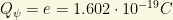
It is generally chosen as fundamental charge the electric charge of the positron (positive charged “electron”). Its value is:

$e=1.602176565(35)\times 10^{-19}C$

where C denotes Coulomb. Of course, if you know about quarks with a fraction of this charge, you could ask why we prefer this one. Really, it is only a question of hystory of Science, since electrons were discovered first (and positrons). Quarks, with one third or two thirds of this amount of elementary charge, were discovered later, but you could define the fundamental unit of charge as multiple or entire fraction of this charge. Moreover, as far as we know, electrons are “elementary”/”fundamental” entities, so, we can use this charge as unit and we can define quark charges in terms of it too. Electric charge is not a fundamental unit in the SI system of units. Charge flow, or electric current, is.

An amazing property of the above 5 constants is that they are “universal”. And, for instance, energy is related with other magnitudes in theories where the above constants are present in a really wonderful and unified manner:

$\boxed{E=N\dfrac{k_BT}{2}=Mc^2=TS=Pc=N\dfrac{h\nu}{2}=N\dfrac{\hbar \omega}{2}=\dfrac{R_Sc^4}{2G_N}=\hbar c k=\dfrac{hc}{\lambda}}$

Caution: k is not the Boltzmann constant but the wave number.

There is a sixth “fundamental” constant related to electromagnetism, but it is also related to the speed of light, the electric charge and the Planck’s constant in a very sutble way. Let me introduce you it too…

6. Coulomb constant. $k_C$ .

This is a second constant related to classical electromagnetism, like the speed of light in vacuum. Coulomb’s constant, the electric force constant, or the electrostatic constant (denoted $k_C$ ) is a proportionality factor that takes part in equations relating electric force between point charges, and indirectly it also appears (depending on your system of units) in expressions for electric fields of charge distributions. Coulomb’s law reads

$F_C=k_C\dfrac{Qq}{r^2}$

Its experimental value is

$k_C=\dfrac{1}{4\pi \varepsilon_0}=\dfrac{c^2\mu_0}{4\pi}=c^2\cdot 10^{-7}H\cdot m^{-1}= 8.9875517873681764\cdot 10^9 Nm^2/C^2$

Generally, the Coulomb constant is dropped out and it is usually preferred to express everything using the electric permitivity of vacuum $\varepsilon_0$ and/or numerical factors depending on the pi number $\pi$ if you choose the gaussian system of units (read this wikipedia article http://en.wikipedia.org/wiki/Gaussian_system_of_units ), the CGS system, or some hybrid units based on them.

H.E.P. units

High Energy Physicists use to employ units in which the velocity is measured in fractions of the speed of light in vacuum, and the action/angular momentum is some multiple of the Planck’s constant. These conditions are equivalent to set

$\boxed{c=1_c=1}$ $\boxed{\hbar=1_\hbar=1}$

Complementarily, or not, depending on your tastes and preferences, you can also set the Boltzmann’s constant to the unit as well

$k_B=1_{k_B}=1$

and thus the complete HEP system is defined if you set

$\boxed{c=\hbar=k_B=1}$

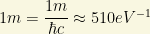
This “natural” system of units is lacking yet a scale of energy. Then, it is generally added the electron-volt $eV$ as auxiliary quantity defining the reference energy scale. Despite the fact that this is not a “natural unit” in the proper sense because it is defined by a natural property, the electric charge, and the anthropogenic unit of electric potential, the volt. The SI prefixes multiples of eV are used as well: keV, MeV, GeV, etc. Here, the eV is used as reference energy quantity, and with the above election of “elementary/natural units” (or any other auxiliary unit of energy), any quantity can be expressed. For example, a distance of 1 m can be expressed in terms of eV, in natural units, as

$1m=\dfrac{1m}{\hbar c}\approx 510eV^{-1}$

This system of units have remarkable conversion factors

A) $1 eV^{-1}$ of length is equal to $1.97\cdot 10^{-7}m =(1\text{eV}^{-1})\hbar c$

B) $1 eV$ of mass is equal to $1.78\cdot 10^{-36}kg=1\times \dfrac{eV}{c^2}$

C) $1 eV^{-1}$ of time is equal to $6.58\cdot 10^{-16}s=(1\text{eV}^{-1})\hbar$

D) $1 eV$ of temperature is equal to $1.16\cdot 10^4K=1eV/k_B$

E) $1 unit$ of electric charge in the Lorentz-Heaviside system of units is equal to $5.29\cdot 10^{-19}C=e/\sqrt{4\pi\alpha}$

F) $1 unit$ of electric charge in the Gaussian system of units is equal to $1.88\cdot 10^{-18}C=e/\sqrt{\alpha}$

This system of units, therefore, leaves free only the energy scale (generally it is chosen the electron-volt) and the electric measure of fundamentl charge. Every other unit can be related to energy/charge. It is truly remarkable than doing this (turning invisible the above three constants) you can “unify” different magnitudes due to the fact these conventions make them equivalent. For instance, with natural units:

1) Length=Time=1/Energy=1/Mass.

It is due to $x=ct$ , $E=Mc^2$ and $E=hc/\lambda$ equations. Setting $c$ and $h$ or $\hbar$ provides

$x=t$ , $E=M$ and $E=1/\lambda$ .

Note that natural units turn invisible the units we set to the unit! That is the key of the procedure. It simplifies equations and expressions. Of course, you must be careful when you reintroduce constants!

2) Energy=Mass=Momemntum=Temperature.

It is due to $E=k_BT$ , $E=Pc$ and $E=Mc^2$ again.

One extra bonus for theoretical physicists is that natural units allow to build and write proper lagrangians and hamiltonians (certain mathematical operators containing the dynamics of the system enconded in them), or equivalently the action functional, with only the energy or “mass” dimension as “free parameter”. Let me show how it works.

Natural units in HEP identify length and time dimensions. Thus $\left[L\right]=\left[T\right]$ . Planck’s constant allows us to identify those 2 dimensions with 1/Energy (reciprocals of energy) physical dimensions. Therefore, in HEP units, we have

$\boxed{\left[L\right]=\left[T\right]=\left[E\right]^{-1}}$

The speed of light identifies energy and mass, and thus, we can often heard about “mass-dimension” of a lagrangian in the following sense. HEP units can be thought as defining “everything” in terms of energy, from the pure dimensional ground. That is, every physical dimension is (in HEP units) defined by a power of energy:

$\boxed{\left[E\right]^n}$

Thus, we can refer to any magnitude simply saying the power of such physical dimension (or you can think logarithmically to understand it easier if you wish). With this convention, and recalling that energy dimension is mass dimension, we have that

$\left[L\right]=\left[T\right]=-1$ and $\left[E\right]=\left[M\right]=1$

Using these arguments, the action functional is a pure dimensionless quantity, and thus, in D=4 spacetime dimensions, lagrangian densities must have dimension 4 ( or dimension D is a general spacetime).

$\displaystyle{S=\int d^4x \mathcal{L}\rightarrow \left[\mathcal{L}\right]=4}$

$\displaystyle{S=\int d^Dx \mathcal{L}\rightarrow \left[\mathcal{L}\right]=D}$

In D=4 spacetime dimensions, it can be easily showed that

$\left[\partial_\mu\right]=\left[\Phi\right]=\left[A^\mu\right]=1$

$\left[\Psi_D\right]=\left[\Psi_M\right]=\left[\chi\right]=\left[\eta\right]=\dfrac{3}{2}$

where $\Phi$ is a scalar field, $A^\mu$ is a vector field (like the electromagnetic or non-abelian vector gauge fields), and $\Psi_D, \Psi_M, \chi, \eta$ are a Dirac spinor, a Majorana spinor, and $\chi, \eta$ are Weyl spinors (of different chiralities). Supersymmetry (or SUSY) allows for anticommuting c-numbers (or Grassmann numbers) and it forces to introduce auxiliary parameters with mass dimension $-1/2$ . They are the so-called SUSY transformation parameters $\zeta_{SUSY}=\epsilon$ . There are some speculative spinors called ELKO fields that could be non-standandard spinor fields with mass dimension one! But it is an advanced topic I am not going to discuss here today. In general D spacetime dimensions a scalar (or vector) field would have mass dimension $(D-2)/2$ , and a spinor/fermionic field in D dimensions has generally $(D-1)/2$ mass dimension (excepting the auxiliary SUSY grassmanian fields and the exotic idea of ELKO fields). This dimensional analysis is very useful when theoretical physicists build up interacting lagrangians, since we can guess the structure of interaction looking at purely dimensional arguments every possible operator entering into the action/lagrangian density! In summary, therefore, for any D:

$\boxed{\left[\Phi\right]=\left[A_\mu\right]=\dfrac{D-2}{2}\equiv E^{\frac{D-2}{2}}=M^{\frac{D-2}{2}}}$

$\boxed{\left[\Psi\right]=\dfrac{D-1}{2}\equiv E^{\frac{D-1}{2}}=M^{\frac{D-1}{2}}}$

Remark (for QFT experts only): Don’t confuse mass dimension with the final transverse polarization degrees or “degrees of freedom” of a particular field, i.e., “components” minus “gauge constraints”. E.g.: a gauge vector field has $D-2$ degrees of freedom in D dimensions. They are different concepts (although both closely related to the spacetime dimension where the field “lives”).

In summary:

i) HEP units are based on QM (Quantum Mechanics), SR (Special Relativity) and Statistical Mechanics (Entropy and Thermodynamics).

ii) HEP units need to introduce a free energy scale, and it generally drives us to use the eV or electron-volt as auxiliary energy scale.

iii) HEP units are useful to dimensional analysis of lagrangians (and hamiltonians) up to “mass dimension”.

Stoney Units

In Physics, the Stoney units form a alternative set of natural units named after the Irish physicist George Johnstone Stoney, who first introduced them as we know it today in 1881. However, he presented the idea in a lecture entitled “On the Physical Units of Nature” delivered to the British Association before that date, in 1874. They are the first historical example of natural units and “unification scale” somehow. Stoney units are rarely used in modern physics for calculations, but they are of historical interest but some people like Wilczek has written about them (see, e.g., http://arxiv.org/abs/0708.4361). These units of measurement were designed so that certain fundamental physical constants are taken as reference basis without the Planck scale being explicit, quite a remarkable fact! The set of constants that Stoney used as base units is the following:

A) Electric charge, $e=1_e$ .

B) Speed of light in vacuum, $c=1_c$ .

C) Gravitational constant, $G_N=1_{G_N}$ .

D) The Reciprocal of Coulomb constant, $1/k_C=4\pi \varepsilon_0=1_{k_C^{-1}}=1_{4\pi \varepsilon_0}$ .

Stony units are built when you set these four constants to the unit, i.e., equivalently, the Stoney System of Units (S) is determined by the assignments:

$\boxed{e=c=G_N=4\pi\varepsilon_0=1}$

Interestingly, in this system of units, the Planck constant is not equal to the unit and it is not “fundamental” (Wilczek remarked this fact here ) but:

$\hbar=\dfrac{1}{\alpha}\approx 137.035999679$

Today, Planck units are more popular Planck than Stoney units in modern physics, and even there are many physicists who don’t know about the Stoney Units! In fact, Stoney was one of the first scientists to understand that electric charge was quantized!; from this quantization he deduced the units that are now named after him.

The Stoney length and the Stoney energy are collectively called the Stoney scale, and they are not far from the Planck length and the Planck energy, the Planck scale. The Stoney scale and the Planck scale are the length and energy scales at which quantum processes and gravity occur together. At these scales, a unified theory of physics is thus likely required. The only notable attempt to construct such a theory from the Stoney scale was that of H. Weyl, who associated a gravitational unit of charge with the Stoney length and who appears to have inspired Dirac’s fascination with the large number hypothesis. Since then, the Stoney scale has been largely neglected in the development of modern physics, although it is occasionally discussed to this day. Wilczek likes to point out that, in Stoney Units, QM would be an emergent phenomenon/theory, since the Planck constant wouldn’t be present directly but as a combination of different constants. By the other hand, the Planck scale is valid for all known interactions, and does not give prominence to the electromagnetic interaction, as the Stoney scale does. That is, in Stoney Units, both gravitation and electromagnetism are on equal footing, unlike the Planck units, where only the speed of light is used and there is no more connections to electromagnetism, at least, in a clean way like the Stoney Units do. Be aware, sometimes, rarely though, Planck units are referred to as Planck-Stoney units.

What are the most interesting Stoney system values? Here you are the most remarkable results:

1) Stoney Length, $L_S$ .

$\boxed{L_S=\sqrt{\dfrac{G_Ne^2}{(4\pi\varepsilon)c^4}}\approx 1.38\cdot 10^{-36}m}$

2) Stoney Mass, $M_S$ .

$\boxed{M_S=\sqrt{\dfrac{e^2}{G_N(4\pi\varepsilon_0)}}\approx 1.86\cdot 10^{-9}kg}$

3) Stoney Energy, $E_S$ .

$\boxed{E_S=M_Sc^2=\sqrt{\dfrac{e^2c^4}{G_N(4\pi\varepsilon_0)}}\approx 1.67\cdot 10^8 J=1.04\cdot 10^{18}GeV}$

4) Stoney Time, $t_S$ .

$\boxed{t_S=\sqrt{\dfrac{G_Ne^2}{c^6(4\pi\varepsilon_0)}}\approx 4.61\cdot 10^{-45}s}$

5) Stoney Charge, $Q_S$ .

$\boxed{Q_S=e\approx 1.60\cdot 10^{-19}C}$

6) Stoney Temperature, $T_S$ .

$\boxed{T_S=E_S/k_B=\sqrt{\dfrac{e^2c^4}{G_Nk_B^2(4\pi\varepsilon_0)}}\approx 1.21\cdot 10^{31}K}$

Planck Units

The reference constants to this natural system of units (generally denoted by P) are the following 4 constants:

1) Gravitational constant. $G_N$

2) Speed of light. $c$ .

3) Planck constant or rationalized Planck constant. $\hbar$ .

4) Boltzmann constant. $k_B$ .

The Planck units are got when you set these 4 constants to the unit, i.e.,

$\boxed{G_N=c=\hbar=k_B=1}$

It is often said that Planck units are a system of natural units that is not defined in terms of properties of any prototype, physical object, or even features of any fundamental particle. They only refer to the basic structure of the laws of physics: c and G are part of the structure of classical spacetime in the relativistic theory of gravitation, also known as general relativity, and ℏ captures the relationship between energy and frequency which is at the foundation of elementary quantum mechanics. This is the reason why Planck units particularly useful and common in theories of quantum gravity, including string theory or loop quantum gravity.

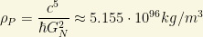
This system defines some limit magnitudes, as follows:

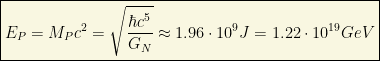
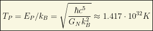
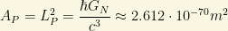
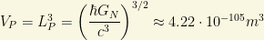
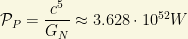
1) Planck Length, $L_P$ .

$\boxed{L_P=\sqrt{\dfrac{G_N\hbar}{c^3}}\approx 1.616\cdot 10^{-35}s}$

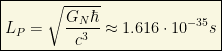
2) Planck Time, $t_P$ .

$\boxed{t_P=L_P/c=\sqrt{\dfrac{G_N\hbar}{c^5}}\approx 5.391\cdot 10^{-44}s}$

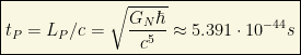
3) Planck Mass, $M_P$ .

$\boxed{M_P=\sqrt{\dfrac{\hbar c}{G_N}}\approx 2.176\cdot 10^{-8}kg}$

4) Planck Energy, $E_P$ .

$\boxed{E_P=M_Pc^2=\sqrt{\dfrac{\hbar c^5}{G_N}}\approx 1.96\cdot 10^9J=1.22\cdot 10^{19}GeV}$

5) Planck charge, $Q_P$ .

In Lorentz-Heaviside electromagnetic units

$\boxed{Q_P=\sqrt{\hbar c \varepsilon_0}=\dfrac{e}{\sqrt{4\pi\alpha}}\approx 5.291\cdot 10^{-19}C}$

In Gaussian electromagnetic units

$\boxed{Q_P=\sqrt{\hbar c (4\pi\varepsilon_0)}=\dfrac{e}{\sqrt{\alpha}}\approx 1.876\cdot 10^{-18}C}$

6) Planck temperature, $T_P$ .

$\boxed{T_P=E_P/k_B=\sqrt{\dfrac{\hbar c^5}{G_Nk_B^2}}\approx 1.417\cdot 10^{32}K}$

From these “fundamental” magnitudes we can build many derived quantities in the Planck System:

1) Planck area.

$A_P=L_P^2=\dfrac{\hbar G_N}{c^3}\approx 2.612\cdot 10^{-70}m^2$

2) Planck volume.

$V_P=L_P^3=\left(\dfrac{\hbar G_N}{c^3}\right)^{3/2}\approx 4.22\cdot 10^{-105}m^3$

3) Planck momentum.

$P_P=M_Pc=\sqrt{\dfrac{\hbar c^3}{G_N}}\approx 6.52485 kgm/s$

A relatively “small” momentum!

4) Planck force.

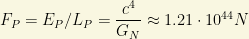
$F_P=E_P/L_P=\dfrac{c^4}{G_N }\approx 1.21\cdot 10^{44}N$

It is independent from Planck constant! Moreover, the Planck acceleration is

$a_P=F_P/M_P=\sqrt{\dfrac{c^7}{G_N\hbar}}\approx 5.561\cdot 10^{51}m/s^2$

5) Planck Power.

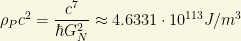
$\mathcal{P}_P=\dfrac{c^5}{G_N}\approx 3.628\cdot 10^{52}W$

6) Planck density.

$\rho_P=\dfrac{c^5}{\hbar G_N^2}\approx 5.155\cdot 10^{96}kg/m^3$

Planck density energy would be equal to

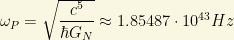
$\rho_P c^2=\dfrac{c^7}{\hbar G_N^2}\approx 4.6331\cdot 10^{113}J/m^3$

7) Planck angular frequency.

$\omega_P=\sqrt{\dfrac{c^5}{\hbar G_N}}\approx 1.85487\cdot 10^{43}Hz$

8) Planck pressure.

$p_P=\dfrac{F_P}{A_P}=\dfrac{c^7}{G_N^2\hbar}=\rho_P c^2\approx 4.6331\cdot 10^{113}Pa$

Note that Planck pressure IS the Planck density energy!

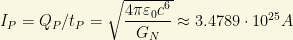
9) Planck current.

$I_P=Q_P/t_P=\sqrt{\dfrac{4\pi\varepsilon_0 c^6}{G_N}}\approx 3.4789\cdot 10^{25}A$

10) Planck voltage.

$v_P=E_P/Q_P=\sqrt{\dfrac{c^4}{4\pi\varepsilon_0 G_N}}\approx 1.04295\cdot 10^{27}V$

11) Planck impedance.

$Z_P=v_P/I_P=\dfrac{\hbar^2}{Q_P}=\dfrac{1}{4\pi \varepsilon_0 c}\approx 29.979\Omega$

A relatively small impedance!

12) Planck capacitor.

$C_P=Q_P/v_P=4\pi\varepsilon_0\sqrt{\dfrac{\hbar G_N}{ c^3}} \approx 1.798\cdot 10^{-45}F$

Interestingly, it depends on the gravitational constant!

Some Planck units are suitable for measuring quantities that are familiar from daily experience. In particular:

1 Planck mass is about 22 micrograms.

1 Planck momentum is about 6.5 kg m/s

1 Planck energy is about 500kWh.

1 Planck charge is about 11 elementary (electronic) charges.

1 Planck impendance is almost 30 ohms.

Moreover:

i) A speed of 1 Planck length per Planck time is the speed of light, the maximum possible speed in special relativity.

ii) To understand the Planck Era and “before” (if it has sense), supposing QM holds yet there, we need a quantum theory of gravity to be available there. There is no such a theory though, right now. Therefore, we have to wait if these ideas are right or not.

iii) It is believed that at Planck temperature, the whole symmetry of the Universe was “perfect” in the sense the four fundamental foces were “unified” somehow. We have only some vague notios about how that theory of everything (TOE) would be.

The physical dimensions of the known Universe in terms of Planck units are “dramatic”:

i) Age of the Universe is about 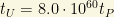$t_U=8.0\cdot 10^{60} t_P$ .

ii) Diameter of the observable Universe is about $d_U=5.4\cdot 10^{61}L_P$

iii) Current temperature of the Universe is about $1.9 \cdot 10^{-32}T_P$

iv) The observed cosmological constant is about $5.6\cdot 10^{-122}t_P^{-2}$

v) The mass of the Universe is about $10^{60}m_p$ .

vi) The Hubble constant is $71km/s/Mpc\approx 1.23\cdot 10^{-61}t_P^{-1}$

Schrödinger Units

The Schrödinger Units do not obviously contain the term c, the speed of light in a vacuum. However, within the term of the Permittivity of Free Space [i.e., electric constant or vacuum permittivity], and the speed of light plays a part in that particular computation. The vacuum permittivity results from the reciprocal of the speed of light squared times the magnetic constant. So, even though the speed of light is not apparent in the Schrödinger equations it does exist buried within its terms and therefore influences the decimal placement issue within square roots. The essence of Schrödinger units are the following constants:

A) Gravitational constant $G_N$ .

B) Planck constant $\hbar$ .

C) Boltzmann constant $k_B$ .

D) Coulomb constant or equivalently the electric permitivity of free space/vacuum $k_C=1/4\pi\varepsilon_0$ .

E) The electric charge of the positron $e$ .

In this sistem $\psi$ we have

$\boxed{G_N=\hbar =k_B =k_C =1}$

1) Schrödinger Length $L_{Sch}$ .

$L_\psi=\sqrt{\dfrac{\hbar^4 G_N(4\pi\varepsilon_0)^3}{e^6}}\approx 2.593\cdot 10^{-32}m$

2) Schrödinger time $t_{Sch}$ .

$t_\psi=\sqrt{\dfrac{\hbar^6 G_N(4\pi\varepsilon_0)^5}{e^{10}}}\approx 1.185\cdot 10^{-38}s$

3) Schrödinger mass $M_{Sch}$ .

$M_\psi=\sqrt{\dfrac{e^2}{G_N(4\pi\varepsilon_0)}}\approx 1.859\cdot 10^{-9}kg$

4) Schrödinger energy $E_{Sch}$ .

$E_\psi=\sqrt{\dfrac{e^{10}}{\hbar^4(4\pi\varepsilon_0)^5G_N}}\approx 8890 J=5.55\cdot 10^{13}GeV$

5) Schrödinger charge $Q_{Sch}$ .

$Q_\psi =e=1.602\cdot 10^{-19}C$

6) Schrödinger temperature $T_{Sch}$ .

$T_\psi=E_\psi/k_B=\sqrt{\dfrac{e^{10}}{\hbar^4(4\pi\varepsilon_0)^5G_Nk_B^2}}\approx 6.445\cdot 10^{26}K$

Atomic Units

There are two alternative systems of atomic units, closely related:

1) Hartree atomic units:

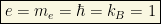
$\boxed{e=m_e=\hbar=k_B=1}$ and $\boxed{c=\alpha^{-1}}$

2) Rydberg atomic units:

$\boxed{\dfrac{e}{\sqrt{2}}=2m_e=\hbar=k_B=1}$ and $\boxed{c=2\alpha^{-1}}$

There, $m_e$ is the electron mass and $\alpha$ is the electromagnetic fine structure constant. These units are designed to simplify atomic and molecular physics and chemistry, especially the quantities related to the hydrogen atom, and they are widely used in these fields. The Hartree units were first proposed by Doublas Hartree, and they are more common than the Rydberg units.

The units are adapted to characterize the behavior of an electron in the ground state of a hydrogen atom. For example, using the Hartree convention, in the Böhr model of the hydrogen atom, an electron in the ground state has orbital velocity = 1, orbital radius = 1, angular momentum = 1, ionization energy equal to 1/2, and so on.

Some quantities in the Hartree system of units are:

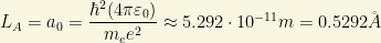
1) Atomic Length (also called Böhr radius):

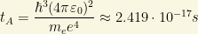
$L_A=a_0=\dfrac{\hbar^2 (4\pi\varepsilon_0)}{m_ee^2}\approx 5.292\cdot 10^{-11}m=0.5292\AA$

2) Atomic Time:

$t_A=\dfrac{\hbar^3(4\pi\varepsilon_0)^2}{m_ee^4}\approx 2.419\cdot 10^{-17}s$

3) Atomic Mass:

$M_A=m_e\approx 9.109\cdot 10^{-31}kg$

4) Atomic Energy:

$E_A=m_ec^2=\dfrac{m_ee^4}{\hbar^2(4\pi\varepsilon_0)^2} \approx 4.36\cdot 10^{ -18}J=27.2eV=2\times(13.6)eV=2Ry$

5) Atomic electric Charge:

$Q_A=q_e=e\approx 1.602\cdot 10^{-19}C$

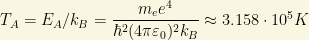
6) Atomic temperature:

$T_A=E_A/k_B=\dfrac{m_ee^4}{\hbar^2(4\pi\varepsilon_0)^2k_B}\approx 3.158\cdot 10^5K$

The fundamental unit of energy is called the Hartree energy in the Hartree system and the Rydberg energy in the Rydberg system. They differ by a factor of 2. The speed of light is relatively large in atomic units (137 in Hartree or 274 in Rydberg), which comes from the fact that an electron in hydrogen tends to move much slower than the speed of light. The gravitational constant is extremely small in atomic units (about 10⁻⁴⁵), which comes from the fact that the gravitational force between two electrons is far weaker than the Coulomb force . The unit length, L_A, is the so-called and well known Böhr radius, a₀.

The values of c and e shown above imply that $e=\sqrt{\alpha \hbar c}$ , as in Gaussian units, not Lorentz-Heaviside units. However, hybrids of the Gaussian and Lorentz–Heaviside units are sometimes used, leading to inconsistent conventions for magnetism-related units. Be aware of these issues!

QCD Units

In the framework of Quantum Chromodynamics, a quantum field theory (QFT) we know as QCD, we can define the QCD system of units based on:

1) QCD Length $L_{QCD}$ .

$L_{QCD}=\dfrac{\hbar}{m_pc}\approx 2.103\cdot 10^{-16}m$

and where $m_p$ is the proton mass (please, don’t confuse it with the Planck mass $M_P$ ).

2) QCD Time $t_{QCD}$ .

$t_{QCD}=\dfrac{\hbar}{m_pc^2}\approx 7.015\cdot 10^{-25}s$

3) QCD Mass $M_{QCD}$ .

$M_{QCD}=m_p\approx 1.673\cdot 10^{-27}kg$

4) QCD Energy $E_{QCD}$ .

$E_{QCD}=M_{QCD}c^2=m_pc^2\approx 1.504\cdot 10^{-10}J=938.6MeV=0.9386GeV$

Thus, QCD energy is about 1 GeV!

5) QCD Temperature $T_{QCD}$ .

$T_{QCD}=E_{QCD}/k_B=\dfrac{m_pc^2}{k_B}\approx 1.089\cdot 10^{13}K$

6) QCD Charge $Q_{QCD}$ .

In Heaviside-Lorent units:

$Q_{QCD}=\dfrac{1}{\sqrt{4\pi\alpha}}e\approx 5.292\cdot 10^{-19}C$

In Gaussian units:

$Q_{QCD}=\dfrac{1}{\sqrt{\alpha}}e\approx 1.876\cdot 10^{-18}C$

Geometrized Units

The geometrized unit system, used in general relativity, is not a completely defined system. In this system, the base physical units are chosen so that the speed of light and the gravitational constant are set equal to unity. Other units may be treated however desired. By normalizing appropriate other units, geometrized units become identical to Planck units. That is, we set:

$\boxed{G_N=c=1}$

and the remaining constants are set to the unit according to your needs and tastes.

Conversion Factors

This table from wikipedia is very useful:

where:

i) $\alpha$ is the fine-structure constant, approximately 0.007297.

ii) $\alpha_G=\dfrac{m_e^2}{M_P^2}\approx 1.752\cdot 10^{-45}$ is the gravitational fine-structure constant.

Some conversion factors for geometrized units are also available:

Conversion from kg, s, C, K into m:

$G_N/c^2$ [m/kg]

$c$ [m/s]

$\sqrt{G_N/(4\pi\varepsilon_0)}/c^2$ [m/C]

$G_Nk_B/c^2$ [m/K]

Conversion from m, s, C, K into kg:

$c^2/G_N$ [kg/m]

$c^3/G_N$ [kg/s]

$1/\sqrt{G_N4\pi\varepsilon_0}$ [kg/C]

$k_B/c^2$ [kg/K]

Conversion from m, kg, C, K into s

$1/c$ [s/m]

$G_N/c^3$ [s/kg]

$\sqrt{\dfrac{G_N}{4\pi\varepsilon_0}}/c^3$ [s/C]

$G_Nk_B/c^5$ [s/K]

Conversion from m, kg, s, K into C

$c^2/\sqrt{\dfrac{G_N}{4\pi\varepsilon_0}}$ [C/m]

$(G_N4\pi\varepsilon_0)^{1/2}$ [C/kg]

$c^3/(G_N/(4\pi\varepsilon_0))^{1/2}$ [C/s]

$k_B\sqrt{G_N4\pi\varepsilon_0}/c^2$ [C/K]

Conversion from m, kg, s, C into K

$c^4/(G_Nk_B)$ [K/m]

$c^2/k_B$ [K/kg]

$c^5/(G_Nk_B)$ [K/s]

$c^2/(k_B\sqrt{G_N4\pi\varepsilon_0})$ [K/C]

Or you can read off factors from this table as well:

and

Advantages and Disadvantages of Natural Units

Natural units have some advantages (“Pro”):

1) Equations and mathematical expressions are simpler in Natural Units.

2) Natural units allow for the match between apparently different physical magnitudes.

3) Some natural units are independent from “prototypes” or “external patterns” beyond some clever and trivial conventions.

4) They can help to unify different physical concetps.

However, natural units have also some disadvantages (“Cons”):

1) They generally provide less precise measurements or quantities.

2) They can be ill-defined/redundant and own some ambiguity. It is also caused by the fact that some natural units differ by numerical factors of pi and/or pure numbers, so they can not help us to understand the origin of some pure numbers (adimensional prefactors) in general.

Moreover, you must not forget that natural units are “human” in the sense you can addapt them to your own needs, and indeed,you can create your own particular system of natural units! However, said this, you can understand the main key point: fundamental theories are who finally hint what “numbers”/”magnitudes” determine a system of “natural units”.

Remark: the smart designer of a system of natural unit systems must choose a few of these constants to normalize (set equal to 1). It is not possible to normalize just any set of constants. For example, the mass of a proton and the mass of an electron cannot both be normalized: if the mass of an electron is defined to be 1, then the mass of a proton has to be $\approx 6\pi^5\approx 1936$ . In a less trivial example, the fine-structure constant, α≈1/137, cannot be set to 1, because it is a dimensionless number. The fine-structure constant is related to other fundamental constants through a very known equation:

$\alpha=\dfrac{k_Ce^2}{\hbar c}$

where $k_C$ is the Coulomb constant, e is the positron electric charge (elementary charge), ℏ is the reduced Planck constant, and c is the again the speed of light in vaccuum. It is believed that in a normal theory is not possible to simultaneously normalize all four of the constants c, ℏ, e, and k_C.

Fritzsch-Xing plot

Fritzsch and Xing have developed a very beautiful plot of the fundamental constants in Nature (those coming from gravitation and the Standard Model). I can not avoid to include it here in the 2 versions I have seen it. The first one is “serious”, with 29 “fundamental constants”:

However, I prefer the “fun version” of this plot. This second version is very cool and it includes 28 “fundamental constants”:

The Okun Cube

Long ago, L.B. Okun provided a very interesting way to think about the Planck units and their meaning, at least from current knowledge of physics! He imagined a cube in 3d in which we have 3 different axis. Planck units are defined as we have seen above by 3 constants $c, \hbar, G_N$ plus the Boltzmann constant. Imagine we arrange one axis for c-Units, one axis for $\hbar$ -units and one more for $G_N$ -units. The result is a wonderful cube:

Or equivalently, sometimes it is seen as an equivalent sketch ( note the Planck constant is NOT rationalized in the next cube, but it does not matter for this graphical representation):

Classical physics (CP) corresponds to the vanishing of the 3 constants, i.e., to the origin $(0,0,0)$ .

Newtonian mechanics (NM) , or more precisely newtonian gravity plus classical mechanics, corresponds to the “point” $(0,0,G_N)$ .

Special relativity (SR) corresponds to the point $(0,1/c,0)$ , i.e., to “points” where relativistic effects are important due to velocities close to the speed of light.

Quantum mechanics (QM) corresponds to the point $(h,0,0)$ , i.e., to “points” where the action/angular momentum fundamental unit is important, like the photoelectric effect or the blackbody radiation.

Quantum Field Theory (QFT) corresponds to the point $(h,1/c,0)$ , i.e, to “points” where both, SR and QM are important, that is, to situations where you can create/annihilate pairs, the “particle” number is not conserved (but the particle-antiparticle number IS), and subatomic particles manifest theirselves simultaneously with quantum and relativistic features.

Quantum Gravity (QG) would correspond to the point $(h,0,G_N)$ where gravity is quantum itself. We have no theory of quantum gravity yet, but some speculative trials are effective versions of (super)-string theory/M-theory, loop quantum gravity (LQG) and some others.

Finally, the Theory Of Everything (TOE) would be the theory in the last free corner, that arising in the vertex $(h,1/c,G_N)$ . Superstring theories/M-theory are the only serious canditate to TOE so far. LQG does not generally introduce matter fields (some recent trials are pushing into that direction, though) so it is not a TOE candidate right now.

Some final remarks and questions

1) Are fundamental “constants” really constant? Do they vary with energy or time?

2) How many fundamental constants are there? This questions has provided lots of discussions. One of the most famous was this one:

http://arxiv.org/abs/physics/0110060

The trialogue (or dialogue if you are precise with words) above discussed the opinions by 3 eminent physicists about the number of fundamental constants: Michael Duff suggested zero, Gabriel Veneziano argued that there are only 2 fundamental constants while L.B. Okun defended there are 3 fundamental constants

3) Should the cosmological constant be included as a new fundamental constant? The cosmological constant behaves as a constant from current cosmological measurements and cosmological data fits, but is it truly constant? It seems to be…But we are not sure. Quintessence models (some of them related to inflationary Universes) suggest that it could vary on cosmological scales very slowly. However, the data strongly suggest that

$P_\Lambda=-\rho c^2$

It is simple, but it is not understood the ultimate nature of such a “fluid” because we don’t know what kind of “stuff” (either particles or fields) can make the cosmological constant be so tiny and so abundant (about the 72% of the Universe is “dark energy”/cosmological constant) as it seems to be. We do know it can not be “known particles”. Dark energy behaves as a repulsive force, some kind of pressure/antigravitation on cosmological scales. We suspect it could be some kind of scalar field but there are many other alternatives that “mimic” a cosmological constant. If we identify the cosmological constant with the vacuum energy we obtain about 122 orders of magnitude of mismatch between theory and observations. A really bad “prediction”, one of the worst predictions in the history of physics!

Be natural and stay tuned!

LOG#068. SM(X): And beyond?

Posted: 2012/12/14 | Author: amarashiki | Filed under: Physmatics, Relativity, The Standard Model: Basics | 3 Comments

1) Is the Higgs like candidate ATLAS/CMS observe a SM Higgs? The Higgs particle is important since it is (like neutrinos) a portal or gate into New Physics. New particles couple naturally to fundamental scalars, so SM deviations can be seen in the Higgs sector better. Indeed, there is a nice table showing the comparison between common Higgs particles and BSM alternative theories in collider physics:

It can, but it could also be an impostor: a technidilaton, a Kaluza-Klein resonance, a dilaton-Higgs, or some other weird particle. However, at current time, it seems to be a SM Higgs.

2) Supersymmetry, a.k.a., SUSY. Double the particle spectrum in order to cancel higher order contributions to the Higgs mass with extra particles ( and fermion “loops”). Does it work? It seems so. It also seems to provide natural DM candidates, but it does not provide any fundamental hint about Dark Energy or the cosmological constant problem. Specially, since we don’t observe (apparently) SUSY at low energy, it has to be broken. If SUSY is broken at higher energy beyon the EW symmetry breaking ( about 246 GeV), it looses some of the main theoretical motivations. Any way, SUSY theories are the most Beyond the Standard Model (BSM) theories. E.g.: supergravity or superstrings in any variant do contain SUSY some variant of SUSY. However, is SUSY realizaed in Nature? We do not know. Yet, we have searched for SUSY since the LEP/TeVatron era, and yet the answer is negative. Of course, it does not mean SUSY does not exist, but as time passes, I see that SUSY is unlikely and unlikely! And let me add that I could hardly admit that some theory like the Minimal Supersymmetric Standard Model (MSSM) could be true, it has too many free parameters. Of course, at current time, you can find some MSSM fit to the SM data, but it is not simple. The MSSM or similar models have the following particle spectrum:

However, some experiments have constrained very hard the SUSY space parameter in order to be consistent with all the current SM data:

Moreover, the LHC has not found SUSY particles yet. ATLAS provides some bounds:

The LHC alone can not rule out the MSSM and lots of SUSY variants, but it is killing some “naive” models and theories. We will need the Linear Collider, a muon collider and/or a Higgs factory in order to kill them all (if possible) with the aid of neutrino experiments, cosmological constraints and likely, further experiments. SUSY can not be excluded but the whole road map of experiments in High Energy Physics can falsify the theory. I am sure of that point. It is only an issue of time (10 or 20 years at most).

3) Technicolor and preonic models. After the Higgs discovery, these models have lost followers. But be aware! If the Higgs particle were composite by fermions, such as technifermions, or it were made of preonic constituents, we could resurrect these theories. However, as long as the Higgs boson shows to be fundamental, and it can be tested, technicolor and preonic models are ruled out (excepting, perhaps, some particular models containing technidilatons or some particle that could mimick the SM Higgs features. It is hard, but it is not impossible to build such a model).

4) Neutrinos. The weirdest particles (and likely the most fascinant) in the SM provide a unique tool and framework to test New Physics and BSM Physics. In particular, neutrinos can be used to test the inner structure of hadrons, and the most exotic processes in the Universe (such a Supernovae/Hypernovae explosions!). There are many reactor neutrino experiments, some accelerator based neutrino oscillation experiments are running and, furthermore, we also have solar neutrino detectors and neutrino telescopes like IceCube and ANTARES. In the nuclear physics domain, we are also studying the deep structure of neutrinos via beta decays. If neutrino are their own antiparticles (note that this option can be realized in the SM known particles only for electrically neutral particles), then neutrinos are Majorana particles. If neutrino are Majorana particles, then neutrinoless double beta decay is possible. Currently, excepting a claim (likely false) by a russian group, there is no evidence for this ultra-weird beta decay. However, it would be a hint of New Physics and BSM physics too.

5) Superstrings and extra dimensional theories. Superstrings (and/or M-theory) are a candidate for the infamous Theory Of Everything (TOE). Feynman opposed himself to this approch in the last years of his life. He used to say he was waiting for the superstring “breaking”. Beyond this particular opinion, the theory has lot of defenders and it has some beautiful features both mathematically and physically. Via model building, you can even derive the SM from the superstrings. But it is not so easy. There are zillions of ways to do it. And nobody knows what select the right geometry/phenomenology from the others. Kaluza-Klein (KK) theories and other more modern theories use extra dimensions just like superstrings but without saying that the whole stuff is made of “strings”. KK theories allow to derive the gravity plus electromagnetism action from a 5 dimensional theory. And the set-up can be generalized for other interactions as well. However, again, there are some mysteries and problems unsolved. Why does a particular KK select a particular geometry/compactification space? What about the Planck scale excitations arising in the KK-states? However, some models with extra dimensions are useful since they can be tested and they provide a model to explain the Higgs mass as a pseudo-Goldstone boson in the extra dimension. It is the so-called Little Higgs theory. Of course, you can also have, beyond strings or KK-particles, arbitrary p-branes (p-dimensional extended objects like membranes and so on). Some extra dimensional scenarios like de ADD (Arkani-Hamed, Dvali-Dmopoulos) large extra dimension picture of gravity plus SM in order to solve the hierarchy problem and/or the celebrated warped brane-world by Randall-Sundrum (the RS model) were a the extra dimension hides itself in a non-factorizable metric.

6) Quantum gravity and Loop Quantum Gravity. Quantum gravity is a complete mystery. However, the supertring theory approach claims to handle with it. Moreover, a parallel and independent approach called Loop Quantum Gravity (LQG) claims to be able to quantize gravity in a non-canonical way using “loop variables”. Loop variables are the analogue for gravity to Wilson loops in non-abelian gauge theories like QCD. LQG provides some predictions like a discrete length, area and volume spectra, and complementary predictions related to the scale where spacetime discretenes appears. However, experimental for Quantum Gravity (QG) and/or LQG is yet lacking (seemingly).

7) CPT and Lorentz invariance violations. Currently, special relativity, General Relativity and Quantum Field Theories like the SM are consistent with Lorentz invariance and CPT invariance. Lorentz invariance is essential to explain any relativistic prediction of High Energy Experiments, and/or, experiments happening to velocities close to the speed of light. Lorentz invariance says that motion is relative and that the speed of light is the upper limit for material particles. However, there are some theories and extensions of the SM that allow Lorentz invariance violations. Even more, there is a whole theoretical framework called the Standard Model Extension (SME) to accomplish these violations and CPT violations. Relativistic local gauge theories are generally built to be CPT invariance. However, they allow for C, CP, P, T, CT, PT violations. In the framework of constructive gauge field theories one can show that local gauge theories are indeed CPT invariant! Then, if we could measure some CPT violating phenomenon, it could hint New Physics/BSM Physics too. SME can handle CPT violating terms in the same way it faces Lorentz violating terms with a unified tool. Note that, even if known Physics imply that Lorentz violations are “equivalent” to CPT violations, in general, it is not true for some BSM theories. Any theory going beyond the SM could manifest itself in different kind of terms, and the elegant way to study these violations is using the SME formalism. Furthermore, some theories BSM like some superstring models or LQG predict that the relativistid dispersion relations of Special Relativity (SR) are modified at high energy. We can test this modified dispersion relationships with HEP experiments in colliders and/or astrophysical observations.

8) Doubly Special/Triply Special (quantum) relativities. There are some interesting modifications of SR from the purely kinematical aspects. These modified relativities introduce a second and even a third “natural scale” beyond the speed of light deformation parameter. This is the reason why are called doubly special relativity and triply special relativity. In the realm of Lie algebras there can not exist, a priori, 4th, 5th,… special relativities. Some predictions of these theories are modified dispersion relationships, relative locality and some exotic uncommon phenomena that could be tested from experiments. Currently, excepting maybe the Dark Energy issue that can be seen as a de-Sitter doubly special relativity, there is no hint of this class of enhanced theories of special relativity.

9) Entanglement and the QM/QFT origins/fundational principles. Quantum Mechanics and QFT are included in the SM. One of the most amusing QM phenomena is “entanglement”. Moreover, QM and/or QFT is a relatively large set of rules that remain to be understood. Some people think that the origin is entanglement via Information Theory and entropy. Other people yet think that QM is an approximation to a classical theory. QM and QFT have been tested up to an incredibly inhuman level of precision in some types of measurements. So, why the SM/QM/QFT works as good? What is wrong if any? Is the entanglement valid also for gravitons despite the fact that gravity IS, apparently, a nonlinear theory? Has QM/QFT a foundational principle like the holographic principle arising from Black Hole Physics, some superstring models, or the gauge/gravity duality seems to point out? If classical and quantum realms are related through dualities, does it mean that Quantum Mechanics could be seen as gravity in some particular background? Does it make sense?

10) Fundamental compositeness. Fermions and bosons, and nothing else even at higher energies? What about spacetime? Are fermions, bosons and spacetime emergent from a deeper structure we can not even imagine yet? What are the black hole microstates?

And there are more questions and likely many new theories and stuff to be discovered yet. But I will finish this thread dedicated to the SM here. I will make a further thread with more advanced topics in the future, when I can introduce the suitable mathematical background and I can be sure that I can explain group theory, fields and quantum fields at some minimum level. But again, that will be another thread! I hope you hava enjoyed my first serious ( somewhat introductory though) series.

May the BSM theories and The Prime Principle be with you too! 😉

LOG#067. SM(IX): Summary.

Posted: 2012/12/14 | Author: amarashiki | Filed under: Physmatics, Relativity, The Standard Model: Basics | Leave a comment

What is the SM? What it does?What is not the SM? What it does not?

1) A local relativistic quantum field theory describing matter-energy and the electroweak and strong interactions up to a distance $10^{-15}-10^{-16}cm$ . It is a “correct”, “effective” (approximate) within known experimental errors and “simple” (in principle not in structure) theory describing almost everything with the exception of the the gravitational force, dark matter and dark energy.

2) After spontaneous symmetry breaking (SSB), the SM lagrangian breaks into:

$\displaystyle{\mathcal{L}=\mathcal{L}_{gauge}+\mathcal{L}_H+\sum_i \overline{\Psi}_i (i\partial\!\!\!/ -m_i-\dfrac{m_i h(x)}{V_0})\Psi_i-}$

$\dfrac{g}{2\sqrt{2}}(J_W^\mu W^{-}_\mu J_W^{\mu \dagger}W^+_\mu) -eJ_Q^\mu A_ \mu -\dfrac{g}{2\cos\theta_W}J_Z^\mu Z_\mu$

3) The SM is a mathematically conistent renormalizable, Yang-Mills gauge field theory in 4 spacetime dimensions.

4) The SM predicts (not only fits) some phenomena tested in experiments. E.g.: the existence and form of the weak neutral currents (NC), the existence and mases of the W and Z bosons, the existence of the charm, the botton and the top quarks (for experts: the existence of such heavy quarks is vindicated the celebrated GIM mechanism).

5) Free parameters. Depending on how you count or select the free parameters for renormalization, they oscillate between 17 and 28 free parameters.

6) There is no explanation or prediction of the fermion masses, which vary over several orders of magnitude, or any of the CKM/PMNS mixing parameters. However, note that the mixing parematers are related to coupling constants rations and then, they are related to the ratios of the masses in the SM somehow, but we do not know how and why.

7) The SM includes but does NOT explain charge quantization: every particle has charges which are proportional to $e/3$ to a high level of precision and accuracy.

8) The gauge structure in the SM is encoded in the gauge group $G_{SM}=SU(3)_C\times SU(2)_L\times U(1)_Y$ . It has 3 separate gauge couplings.

9) The electroweak sector/piece of the SM is chiral and parity violating. It also breaks charge conjugation and CP symmetry as well.

10) There are 3 and only 3 families or generations. Two of them seems to be heavier copies of the first family. That is, if we set the fundamental or prime family as the one formed by:

$(e,\nu_e, u, d)$

Then the remaining 2 generations are $(\mu, \nu_\mu, c,s)$ and $(\tau, \nu_\tau, t, b)$ . The SM gives NO explanation of why the additional 2 generations exist, and of course, the SM gives no explanation of any of the structure and number of these and further families.

11) Higgs particles/bosons. The minimal SM predicts an elementary Higgs field to generate fermion masses and the gauge boson masses for the W and Z bosons. The Higgs particle mass should not be too different from the W or Z mass for the total SM consistency, i.e., the SM predicts that $M_H=\mathcal{O}(M_Z)\sim \mathcal{O}(M_W)$ . Theoretical arguments could suggest the existence of low energy SUSY in order to explain how the Higgs mass avoids to receive large renormalizations to its mass. This argument uses cancellation or interference between Feynman diagrams. However, in spite of the fact the Higgs have been discovered this year (2012), we have not found evidence for supersymmetry (SUSY) yet. A broken high-energy SUSY looses some of the appealing for explaining the low Higgs mass and/or solving the hierarchy problem between the electroweak scale and the Planck scale.

12) The existence of generations, the structure of masses and mixing parameters, both in the quark and lepton sectors, suggest the existence of additional “flavor symmetries”: they can be “horizontal” local gauge symmetries or global discrete flavor symmetries.

13) The complex structure of the gauge sector in the SM and complementary experimental and theoretical evidences suggest that the local gauge symmetry group $G_{SM}$ should be embedded into a larger gauge group. It is called the Grand Unification, and theories like these providing an initial gauge group are called Grand Unified Theories or GUT. They would be truly unified theories of electroweak and strong interactions and, likely, the Theory Of Everything (TOE) if we include the gravity into the gauge framework. However, and unfortunately, gravity is NOT a (at least normal) gauge theory. Some particular elections of GUT groups like $SU(5), SO(10), E_8\times E_8, SO(32),...$ are well known in the literature and they do have some predictions that can be tested in the LHC and hopefully additional experiments/observations.

14) Axions and the strong CP problem. Currently, the QCD sector does NOT allow for pure CP violations. However, on theoretical arguments, the SM lagrangian can be complemented with the so-called theta term piece, a pure QCD CP violating lagrangian piece:

$\mathcal{L}_\theta=\dfrac{\theta}{32\pi^2}g_s^2 F\tilde{F}$

and where we have defined the dual field strength

$\tilde{F}_{\mu\nu}=\dfrac{1}{2}\epsilon_{\mu\nu\alpha\beta}F^{\alpha\beta}$

The theta term breaks the P, T and CP symmetries in the QCD sector. Of course, CP symmetry in the QCD sector can be measured experimentally. This term, if it were proved to exist, it would be very tiny since $\theta<10^{-10}$ and it would induce an electric dipole moment $d_N$ to the neutron. The rather stringent limits on the dipole moment provide the previous bound. The smallness of this parameter is called the strong-CP problem and one simple solution (but it is not easy to test at all) is the so-called Peccei-Quinn mechanism and the existence of an extra and additional global symmetry $U(1)_A$ imposed by the theory in such a way that $\theta$ becomes a dynamical variable rather than a constant and it would have a zero value at the minimum of the (Higgs) potential. It also implies the existence of a new (pseudo)scalar particle called the axion. Laboratory, astrophysical and cosmological tests have constrained only a very small window $10^8-10^{12}$ GeV for the Peccei-Quinn scale or the ultralow energy(mass) axion for the axion mass scale (microGeV or even lower) at which the $U(1)_A$ symmetry is broken.

15) The SM and gravity are unrelated. Gravity is not fundamentally unified with the electroweak and strong interactions in the SM. In fact, there is no quantum theory of gravity at current time, only some candidates and temptative (highly speculative) theories.

16) The cosmological constant in the Eisntein’s field equations for gravity can be thought as a vacuum energy. The vacuum expectation value of any scalar Higgs-like field generates indeed a cosmological constant:

$<0\vert V\vert 0>=-\dfrac{\mu^4}{4\lambda}$

when we evaluate such a quantity at the minimum of the potential. It has a large value when the theory couples to gravity due to the fact that a constant energy density IS EQUIVALENT to a cosmological constant. The cosmological constant can be written then as:

$\Lambda_{cosmo}=\Lambda_{bare}+\Lambda_{SSB}$

and where $\Lambda_{bare}$ is the primordial cosmological constant ( the value of the vacuum energy in the absence of SSB) and $\Lambda_{SSB}$ is the term or cosmological constant generated after SSB by the own Higgs mechanism. We have, in the most optimistic scenario, that:

$\vert \Lambda_{SSB}\vert =8\pi G_N \vert <0\vert h \vert 0>\vert \sim 10^{50}\vert \Lambda_{obs}\vert$

It is about 50 or 60 orders of magnitude bigger than the observed cosmological constant (coming from cosmological observations). This is the biggest problem in theoretical physics and likely one of the worst “predictions” of any theory. It remind us the infamous ultraviolet catastrophe in the XIX century though. We hope to solve this formidable problem in the near future somehow. Technically, we could solve the problem naively by adding a new extra term $+\mu^4/4\lambda$ to V, in such a way that V were equal to zero at the minimum. However, such a naive procedure fails. With our current knowledge of the symmetries of Nature, there is no reason to relate the bare cosmological constant and the SSB cosmological constant. That is, the energy density induced by Higgs potential after SSB is many, many orders of magnitude larger than the experimental upper limit. This is called the cosmological constant problem.

Some solutions to this hard problem involve:

i) Using Kaluza-Klein theories in 5 or higher dimensions.

ii) Supergravity theories. These theories of local supersymmetry including gravity solve partially the problem. They can solve the cosmological constant problem but they don’t explain what is the theory of quantum gravity or even we ignore yet if supergravity (SUGRA) theories are renormalizable! Therefore, in current time, they don’t provide any obvious solution to the cosmological constant problem at the fundamental level (it goes beyond the numerical values, as the previous explanations show).

iii) Superstring theory/M-theory/Brane-worlds. They are a wide class of theories that unify gravity and the remaining interactions. It may yield to finite (renormalization free) theories of gravity and quantum gravity or every fundamental interaction. It is not clear yet if they can solve the cosmological constant problem at all!

17) The SM does not say what Dark Matter/Dark Energy are and/or what are they made of. We do know they are stuff we can not explain with the SM. In fact, it seems that the observable Universe that we do understand is at most a ridiculous 5% of the whole Universe. It is puzzling and pushing to go beyond the Standard Model:

18) The origin of the Higgs mass value is a free parameter in the SM, and too, its couplings to the fermions. Then, the origin of the Higgs coupling to fermions is also unknown. Then, the SM can not explain the origin of mass at fundamental level.

19) The Universe is likely made of matter mainly. The SM does not explain why we don’t observe antimatter in the same proportion. This is sometimes called the antimatter problem or the baryon asymmetry problem.

20) The SM predicts a null mass for neutrinos. The fact that neutrinos oscillate was one of the first experimental evidences, added to Dark Matter/Dark Energy and other phenomena, that the SM is not the whole story. The structure of neutrino oscillations via the PMNS matrix is essentially the opposite to the quark mixing. It seems that neutrino oscillations happen with maximal or almost maximal mixing, while the quark mixing happens with almost null mixing (or very soft mixing). We can not understand these mixing patterns in the SM.

21) The cosmic ray enigma. Cosmic rays hit Earth and produce particles we can detect with modern detectors. The cosmic ray energy primaries or the origin of the particle cascades we observe is a complete mystery, but we do know they have an incredible energy, PeV or higher! What is the mechanism of production of cosmic rays? What are primary cosmic rays? We can not know yet but we have some cool experiments working on that issue.

22) The neutrino is the lightest particle but, how many TOTAL neutrino species do exist? Experimentally we do know that there are 3 light neutrino species. But cosmological measurements allow for a little higher number of neutrino species. Is there a sterile neutrino? Could it be causing some of the anomalies we observe in DM and neutrino detection experiments? Is the neutrino a Majorana particle?

23) Is the renormalization procedure necessary? Renormalization has been imposed as a physical requirement but we don’t understand if Nature does renormalization or if renormalization is a mere tool to provide finite answers.

And there are many other questions, some quite technical, that I will not review here, unless you consider them important. Let me know if you know some additional and interesting SM feature/issue or enigma…

Let the SM be with you!

LOG#066. SM(VIII): tests.

Posted: 2012/12/14 | Author: amarashiki | Filed under: Physmatics, Relativity, The Standard Model: Basics | Leave a comment

The weak scale and the weak angle

The Fermi constant is defined through a beautiful and simple mathematical formula:

$\dfrac{G_F}{\sqrt{2}}=\dfrac{g^2}{8M_W^2}$

This formula for the Fermi constant was very important in the long path towards the EW unification since knowing the Fermi constant allows to guess or estimate the value of the W-mass! Moreover, this constant is also determined independently by experimental muon lifetime, and it yields

$G_F=1.16639(2)\cdot 10^{-5}GeV^{-2}$

The weak scale or equivalently the v.e.v. of the physical Higgs field is given by:

$V_0=\dfrac{2M_W}{g}=\left(\sqrt{2}G_F\right)^{-1/2}\approx 246 GeV$

Similarly, we also have a relation between the electric charge and the weak coupling constant via the Weinberg angle

$e=g\sin\theta_W$

To the lowest order (tree level in QFT calculations), the W-boson mass and the Z-boson mass are related

$M_W=M_Z\cos\theta_W\sim \dfrac{(\pi \alpha/\sqrt{2}G_F)^{1/2}}{\sin\theta_W}$

where the electromagnetic fine structure constant is

$\alpha^{-1}_{EM}\approx 137.036$

Experimentally, the Weinberg angle (more precisely its sine or cosine) is determined experimentally from the neutral current scattering experiments, and they provide

$\sin^2\theta_W\approx 0.23$

The Higgs mass: limits and 2012 discovery

Before 2012, theoretical physicists had only theoretical hints about the possible Higgs mass values. The Higgs mass was not predicted by the SM, BUT some general principles based on QM, QFT and preliminary results in collider physics provided the next bounds:

1) We knew experimental lower limits $M_H\geq 114 GeV$ and $M_H\leq 200 GeV$ from LEP (CERN) , CDF (FermiLAB, TeVatron), and the precision measurements of the SM observables, that strongy pointed out towards a “low Higgs mass”.

2) There were strong and theoretical bounds in the “very low” Higgs mass range $0-10GeV$ . Despite the fact they depended on the top quark mass, they strongly suggested that the Higgs mass could not be “very low” in energy. It would have been detected!

3) Some general arguments for strongly coupled Higgs particles, related to the Higgs-self-couplin $\lambda$ strongly suggested that the Higgs particle could not be heavier than $\sim 1 TeV$ .

4) Unitarity in the s-channel scattering for the Higgs bosons suggested that the Higgs boson could not be heavier than $\sim 800GeV$ .

There were some other highly technical bounds on the Higgs mass, but I am not going to discuss it here. There are plenty of books and lectures covering that topic. I am only interested in the master lines of the Higgs hunters…Until this wonderful year. 2012 will be remembered, and this summer particularly, due to the discovery of the Higgs particle ( or something that looks like a Higgs boson, but we have to wait for that claim) by ATLAS and CMS, the two main collaborations in the LHC(Large Hadron Collider, for short). The LHC, a 27 Km hadron-hadron (proton-proton) collider claimed this summer they have found a new boson particle or “resonance” around the mass:

$M_H\approx 125-127GeV$

It is consistent with theoretical and previous experiments/tests but…What value do you prefer? A cubic Higgs mass value $M_H=5^3 GeV$ ? Maybe a magical number like $M_H=126$ GeV?Or maybe you prefer…A prime number like $M_H=127GeV$ . Well, I prefer prime numbers (like the W and Z bosons, closely to 79 and 91 respectively in GeV units), so I like the Higgs mass to be $127 GeV$ ! Indeed, 127 is close to 128, and 128 is also interesting since it is almost the inverse of the electromagnetic fine structure constant at the Z-pole mass! If we are tempted to related couplings to masses as they seem to be from mixing and ratios, this is a deep result or perhaps another extraordinary coincidence!

Moreover, in the end of the 2012 we have obtained strong suggestions that the 127 GeV particle has spin zero and it is very likely to be parity even! Spin zero is what we would expect from a SM Higgs and it would rule out weird spin 2 variants like some extra-dimensional impostors or Kaluza-Klein resonances and similar “cousins”. Being parity even, it also rules out some weird alternative beyond the Standard Model. So, it seems that whatever the New Physics is really very well hidden from our common eyes and vision. At least, till now. In summary, neglecting some disturbances in the ATLAS and CMS experiments, probably some systematic error, every data collected until 2012 is consistent with a SM Higgs. Are you worried as a SUSY/string believer? Perhaps you should not but data can not be denied! 😉 SUSY can hardly be the answer to the EW-Planck hierarchy problem if SUSY is broken. If it(SUSY) is broken at high energy it can not be the explanation of why the Higgs mass is light since it should receive a $\mathcal{O}(M_{SUSY}^4)$ correction that can not be easily explained without a fine-tuned SUSY. If it is not SUY, then what protects the Higgs mass to receive quantum corrections to its mass? Likely, it is one of the most appealing questions that the current SM leaves unsolved!

Quark masses

From the 2012 PDG booklet we obtain:

$m_u=2.3^{+0.7}_{-0.5}MeV$ $m_d=4.8^{+0.7}_{-0.3}MeV$ $m_s=95\pm 5MeV$

$m_c=1.274\pm 0.025GeV$ $m_b(\overline{MS})=4.18\pm 0.03 GeV$ $m_b(1S)=4.65\pm 0.03GeV$

Moreover, direct measurements provide $m_t=173.5\pm 0.6\pm 0.8 GeV$ and minimal substraction $\overline{MS}$ from cross-section measurements give $m_t=160^{+5}_{-4}GeV$ .

We compare these values with the known fundamental masses for leptons:

$m_e= 0.510998928\pm 0.000000011MeV$

$m_\mu=105.6583715\pm0.0000035MeV$

$m_\tau=1776.82\pm 0.16 MeV$

Current values for neutrino masses are now known beyond experimental and theoretical bounds.

Further experimental tests

The charged current interactions have ben succesfully tested both, experimentally and theoretically. Moreover, CC interactions have been tested in weak decays:

1st. Decays involving kaons, hyperons, heavy quarks, muons and tau particles.

2nd. Precision measurments of $\beta$ decays, and/or decays from $\mu, \tau$ particles are a sensitive probe of extended gauge groups involving right-handed currents and other types of new physics associated with new particles that we have not observed yet.

3rd. Tests involving the CKM matrix are important tools for a 4th generation (or higher) existence. It is also important if some new family or some new exotic fermion/interaction arises. Every test that has been done till current time (circa end of 2012) shows that the CKM matrix is unitary and “almost” the unit matrix.

4th. Neutrino scattering processes have been studied:

$\nu_\mu e\rightarrow \mu^- \nu_e$

$\nu_\mu n\rightarrow \mu^- p$

$\nu_\mu N\rightarrow \mu^-X$

Neutrinos, in particular neutrino-hadron collisions, are used as a proe of the inner structure of hadrons and QCD. Neutrino are neutral particles that only interact through the weak interaction and likely the gravitational force, so we can use them as microscopes to see the inner hadron structure.

5th. The mass difference between two kaon species $K_L, K_S$ ,i.e., $M_{K_S}-M_{K_L}$ is a test of CP violation in neutral kaon systems. In addition to it, it is also a test of $B\overline{B}$ -mixing.

Weak interactions and their CC and NC parts were discovered at CERN in 1973 (via the Gargamelle bubble-chamber collaboration). Since then, they have been tested successfully in a large set of experiments. Extra empirical evidence from the EW sector and its CC-NC interactions are provided by:

1) Reactions $\nu e\rightarrow \nu e$ , $\nu N\rightarrow \nu N$ $\nu N\rightarrow \nu X$

where N denotes a “nucleon” state and X an arbitrary set of particles with allowed quantum numbers.

2) Polarized electron-nuclei scatterin: $e^{\uparrow \downarrow}D\rightarrow eX$

3) Parity (and charge) violation experiments in atomic physics.

4) Electron-positron collisions at the Z-pole mass $M_Z$ , or energies $E=M_Zc^2$ , at LEP (before the LHC current era).

Remark: the self-interactions of the gauge bosons in the SM are PREDICTED by the underlying gauge invariance and they are tested experimentally. Experimental evidence for these self-interactions are, for example, processes like

$e^-e^+\rightarrow W^+ W^-$

This class of reactions were seen at LEP II and they are being observed at the LHC. There are three main diagrams for this collision. I mean Feynman diagrams. A technique that I should explain, but not today, as well. Two of them involve the 3-point interaction between a photon or Z boson and the W⁺W⁻ bosons.

After the Higgs-like particle discovery, one of the main tasks of physicists in the LHC is to determine their couplings to the SM fermions and to see IF the Higgs interaction vertices and the observed phenomenology match.

Neutrino oscillations and masses

In 1998, the SuperKamiokande neutrino detector and later, independently, the SNO experiment determined for the first time that neutrinod do indeed flavor “oscillate” or “change” using solar neutrinos, i.e., SuperKamiokande and SNO observed the neutrinos emitted by the Sun, and they conclude they have mass. During the years 2001-2005, neutrino oscillations were studied for the first time at a “reactor experiment” called KamLAND, at Japan, measuring the neutrinos emitted by the different nuclear reactors from the country. They gave the best estimate of the difference in the squares of the neutrino masses. In May 2010, it was reported that physicists from CERN and the Italian National Institute for Nuclear Physics, in Gran Sasso National Laboratory, had observed for the first time a transformation in neutrinos in an accelerator experiment, providing further evidence that neutrino do have mass. Before 2012, the analogue matrix to the CKM matrix, the PMNS matrix, was determined up to one angle, the so-called $\theta_{13}$ . In 2012, this year, the chinese experiment in Daya-Bay (a reactor experiment) and independently later by the south-korean reactor experiment RENO have provided evidence for a non-null and “large” $\sin^2\theta_{13}$ . It has been confirmed by independent experiments. Here you are a nice summary with the last mixing angle they obtained

We do know that neutrino have mass, a fact that is NOT the predictions of the SM. Indeed, the SM “predicts” massless neutrinos. Then, massive neutrinos are strong hints of new physics, whatever it is! However, their absolute scale is not known. We even ignore if neutrinos are even a weirder type of spinor fields called Majorana fields (essentially fermions that are their own antiparticles, unlike the other SM fermions). We have not observed (yet) CP violations in the leptonic sector, but the structure of the now “almost” complete PMNS matrix suggests that they have to exist. Furthermore, we do not know what type of spectrum neutrinos have (normal, inverted or quasidegenerated) or if there are heavy-right handed neutrinos (if they exist they are very massive and uncharged under the SM gauge group!) or sterile neutrinos ( neutrino species, not necessarily right-handed) uncharged under the SM gauge group. Neutrinos are the most mysterious particles of this Universe (if we neglect the graviton, the axion and other exotic particles whose probable existence has not been proved yet!).

The strongest upper limit on the masses of neutrinos comes from cosmological measurements:

1) The Big Bang model predits that there is a fiexe ratio between the number of neutrinos and the number of photons in the cosmic microwave background or CMB. If the total energy of neutrinos surpassed an average of

$m_\nu\leq 50eV$

per neutrino, or any number of this order of magnitude, there would be so much mass in the Universe that it would collapse. It is not collapsing. Even worst, supernovae IA measurements and complementary observations show that the Universe is expanding with an increasing velocity and positive acceleration! This is known as well from 1998…So, the Universe is not collapsing and the rate of the expansion is accelerating. Puzzling and mysterious stuff!

2) Cosmological data, such as the CMB radiation, galaxy clusters and the so-called Lyman-alpha forest indicate that the sum of the neutrino masses must be less that 1 eV ( the bounds are generally model dependent but there are stronger and softer bounds to this reference value of 1eV).

3) In 2009, data from gravitational lensing of a galaxy cluster also suggested a 1-2 eV upper mass bound for the neutrino species.

By the other hand, from the controlled measurements of solar neutrinos, reactor experiments and accelerator experiments ( specially those coming from solar, atmospheric and reactor/accelerator based experiments are crucial) provide some crucial mass differences for the neutrino species in the SM:

1) In 2005 KamLAND provided the estimate

$\Delta m_{21}^2=0.000079eV^2$

2) MINOS experiment (accelerator based neutrino experiment, type long-baseline) provided

$\Delta m_{32}^2=0.0027eV^2$

These data are being improved now, since the neutrino branch of the SM is a very active area of research and it uses very different methods in order to try to determine the neutrino mass absolute spectrum, its character and the spinorial nature of the neutrino field, yet uncovered (circa end of 2012). Such experiments include:

1) Nuclear beta decay (KATRIN, MARE,…).

2) Neutrinoless double beta decay (e.g., GERDA, CUORE/CUORICINO, NEMO-3, and many others).

3) Neutrino telescopes (IceCube, ANTARES,…)

Neutrinos are alive! 🙂 But let the Higgs bosons be with you!

Stay tuned!

LOG#065. SM(VII): phenomenology.

Posted: 2012/12/14 | Author: amarashiki | Filed under: Physmatics, Relativity, The Standard Model: Basics | Leave a comment

The above picture is a cool mind map by the cosmologist and particle physicist Sean Carroll. It summaries somehow the phenomenological charges of the Standard Model plus the gravitational sector we do not know at quantum level.

Physical Higgs sector

The Higgs field $\varphi$ is a field with TWO complex components, or equivalently if you want, FOUR real components in a suitable basis. It has 4 total degrees of freedom (DOF) from the real viewpoint. Three of these DOF are used in the SSB mechanism of mass generation via the gauge fields. Sometimes we say that those 3 DOF are “eaten up” by the Goldstone bosons. The final result is that we have a real scalar field! And the vacuum expectation value (or v.e.v.) is not zero! Then, we can write the Higgs field in the unitary gauge to be:

$\varphi (x)=\dfrac{1}{2}\begin{pmatrix}0\\ V_0+h(x) \end{pmatrix}$

where we have defined the physical Higgs field $h(x)$ and where we have $<h(x)>=0$ . The quantum excitations of the Higgs field are called the Higgs bosons. These particles are predicted by the SM, so we have to find them experimentally. In this year, one ( if not the most) of the most important achievements is the finding of the Higgs boson by the LHC. It was reported by the LHC, during the summer, and it was confirmed independently by the two main collaborations of this wonderful machine/collider: ATLAS and CMS. It deserves the Nobel Prize such a discovery but I will not tell him my opinion about who and when are going to win the prize, or who or when should win it.

By the other hand, using the above equation for the physical Higgs field, we can rewrite the Yukawa pieces into “physical Yukawa pieces”:

$\boxed{\displaystyle{\mathcal{L}_{\mathcal{YUK}}=-\sum_{fermions}m_f\overline{\Psi}_f\Psi_f\left(1+\dfrac{h}{V_0}\right)}}$

The coupling constant is, thus, proportional to the fermion mass through the physical Higgs field! We can make the following split

$\mathcal{L}_{\mathcal{YUK}}+\mathcal{L}_\varphi=\mathcal{L}_{mass}+\mathcal{L}_h$

We would obtain the fermion mass terms as follows:

$\displaystyle{\mathcal{L}_h=-\dfrac{1}{2}(\partial h)^2-\dfrac{1}{2}m_h h^2-\sum_{fermions}\dfrac{m_f}{V_0}\overline{\Psi}_f\Psi_f h+\dfrac{M_Z^2}{V_0}Z_\mu Z^\mu h+\dfrac{2M_W^2}{V_0}W_\mu^+ W^{\mu -}h}$

$\displaystyle{-\dfrac{m_h^2}{2V_0}hhh-\dfrac{m_h^2}{8V_0^2}hhhh+\dfrac{m_W^2}{2V_0^2}W_\mu^+ W^{\mu -}hh+\dfrac{m_Z^2}{2V_0^2}Z_\mu Z^\mu hh}$

This lagrangian corresponds to the so-called Higgs sector of the SM. The physical Higgs field is massive and it interacts with itself and with the massive weak interacting bosons, i.e., it only interacts with the Z and W bosons. If you want to put it in words, the Higgs field is “transparent” for the EM photon field and the QCD gluon fields but it acts like some kind of nonlinear medium with the remaining (and massive) electroweak gauge bosons, and for the remaining fermions fields as well. That is, fermion fields feel the Higgs field and acquire mass as well via the SSB-Higgs mechanism. Some tree level Higgs diagrams are

The above two diagrams were important in Tevatron, the proton-antiproton Fermilab collider. Moreover, we also have, e.g., the interaction vertices:

Fermion mass matrices

The Yukawa interaction in the unitary gauge becomes

$\boxed{\displaystyle{-\mathcal{L}_{\mathcal{YUK}}\rightarrow \sum_{m,n=1}^{F}\overline{u}^0_{mL}\Gamma^u_{mn}\left(\dfrac{V_0+h(x)}{\sqrt{2}}\right)u^0_{mR}+(d,e)\mbox{-Terms}+\mbox{h.c.}}}$

$\boxed{-\mathcal{L}_{\mathcal{YUK}}=\overline{u}^0_L (M^u+h^uh(x))u^0_R+(d,e)\mbox{-Terms}+\mbox{h.c.}}$

and where we have written

$u^0_L=\begin{pmatrix}u^0_{1L} & u^0_{2L} & \cdots & u^0_{FL}\end{pmatrix}$

This vector is a F-component array (column vector), and we have an analogue expression for $u^0_R$ . By the other hand, $M^u$ is a $F\times F$ fermion mass matrix:

$M^u=\dfrac{\Gamma^u_{mn}V_0}{\sqrt{2}}$

It is induced by SSB ( Spontaneous Symmetry Breaking) and

$h^u=\dfrac{M^u}{V_0}=\dfrac{gM^u}{2M_W}$

is the so-called Yukawa coupling matrix.

Remark: The Yukawa coupling matrix express fermion mass terms as functions of the physical higgs mass and its corresponging Higgs-fermion coupling, or equivalently, the Yukawa coupling matrix is related to the Higgs v.e.v. and/or the higgs-coupling and the electroweak boson mass. A truly remarkable fact!

Remark(II): In general the Yukawa coupling matrix is NOT diagonal, hermitian or even symmetric! To identify the physical particle content it is necessary to diagonalize $M$ by some unitary transformations $A_L$ and $A_R$ on both sides (right and left) and onto the left-handed and right-handed fermion fields. In the special case that $M$ is chosen to be hermitian, we can take

$A_L=A_R$

and thus

$A_L^{\dagger u} M^u A_R^{u}=M_D^u=\begin{pmatrix}m_u & 0 & 0\\ 0 & m_c & 0\\ 0 & 0 & m_t\end{pmatrix}$

is a completely diagonal matrix with eigenvalues equal to the physical masses of the quark triplet $(u, c, t)$ with charge $2/3$ . Similarly, we can perform the following transformations:

$A_L^{\dagger d}M^d A_R^d=M^d$

$A_L^{\dagger e}M^e A_R^e=M_D^e$

The mass eigenstates are defined via unitary matrices as:

$u_L=A_L^{\dagger u}u_L^0=(u_L, c_L, t_L)^T$

and similarly for

$u_R=A_R^{\dagger u}u^0_R$

$d_{L,R}=A_{L,R}^{\dagger d}d^0_{L,R}$

$e_{L,R}=A_{L,R}^{\dagger e}e^{0}_{L,R}$

In terms of the charged leptonic unitary transformation, we can choose

$\nu_L=A_L^{\dagger e}\nu_L^0$

Indeed, we define the neutrino fields $\nu_e, \nu_\mu, \nu_\tau$ as the weak interaction partners of the lepton triplet $e, \mu, \tau$ .

Higgs-Fermion couplings

The Higgs-fermion interactions are characterized by the following lagrangian piece:

$\boxed{\displaystyle{\mathcal{L}_{\mathcal{YUK}}=\sum_i \overline{\Psi}_i \left( -m_i-\dfrac{gm_i}{2M_W}h(x)\right)\Psi_i}}$

The Higgs-fermion coupling has some interesting features:

1) The coupling of the physical Higgs boson to the ith fermion is given by a coefficient $gm_i/2M_W$ . It is very small in general, and it is only “large” for the top quark.

2) The coupling Higgs-fermion is diagonal in the “flavor”-space: there is just one and only one Yukawa matris for every type of fermion, so the mass and the Yukawa matrices are diagonalized by the same transformations.

CKM matrix: W-fermion interaction vertices

The W-bosons interact with fermions via weak interaction, through a lagrangian called “charged current” (CC) lagrangian:

$\boxed{\mathcal{L}_{CC}=-\dfrac{g}{2\sqrt{2}}\left(J_W^\mu W_\mu^-+J_W^{\mu \dagger}W_\mu^+\right)}$

The “weak charge-raising current” can be showed to be:

$\displaystyle{J_W^{\mu \dagger}=\sum_{m=1}^F\left[\overline{v}^0_m \gamma^\mu (1-\gamma_5)e^0_m+\overline{u}^0_m (1-\gamma_5) d^0_m\right]}$

or equivalently

$J_W^{\mu \dagger}=\begin{pmatrix}\overline{\nu}_e & \overline{\nu}_\mu & \overline{\nu}_\tau\end{pmatrix}\gamma^\mu (1-\gamma_5)\begin{pmatrix}e^-\\ \mu^-\\ \tau^-\end{pmatrix}+\begin{pmatrix}\overline{u} & \overline{c} & \overline{t}\end{pmatrix}\gamma^\mu (1-\gamma_5)V\begin{pmatrix}d\\ s\\ b\end{pmatrix}$

In fact, this structure for $J_W^{\mu \dagger}$ owns what theoretical physicists call $V-A$ , (vector-axial vector, or vector-pseudovector), form. This structure is essential in order to provide an explanation of parity violation experiments, charge violation experiments and CP violations. Indeed, the CP violations in the EW sector are known to be maximally violated experimentally. The mismatch between unitary transformations for those states that relate the weak and the mass eigenstates for the up-down quark types lead to the existence of the $F\times F$ unitary matrix

$V\equiv A_L^{u\dagger}A_L^{d}$

in the above weak current. This is the CKM (Cabibbo-Kobayashi-Maskawa) or quark mixing matrix matrix. Experimentally, it is known that the CKM is very close to the unit matrix. By the other hand, for instance, if we make V with $F=2$ , i.e., two families or generations, V is written as

$V=\begin{pmatrix}\cos \theta_c & \sin\theta_c\\ -\sin\theta_c & \cos\theta_c\end{pmatrix}$

with $\sin\theta_c\approx 0.22$ , from experiments neglecting the 3rd family. $\theta_c$ is called the Cabibbo angle, and despite the fact of being two-flavored, the F=2 toy model provides a good approximation to the weak interactions of the quarks u, d, s, an c (up, down, strange, charm).

If we go to the complet F=3 case that is realized in the complete SM and, it seems, in Nature/the Physical Realm, we have the full F=3 CKM matrix given by:

$V=V^{CKM}=\begin{pmatrix}V_{ud} & V_{us} &V_{ub}\\ V_{cd} & V_{cs} & V_{cb}\\ V_{td}& V_{ts} & V_{tb}\end{pmatrix}$

The matrix elements are generally complex numbers (it implies CP-viotating “phases”!) and there are some common parametrization of the above matrix in the literature. I am not going to discuss mixing in detail here today, so you will have to wait if you want to see me how to explain quark and lepton mixing, and the structure hidden in their “oscillations”. In fact, we do know that there is a leptonic mixing analogue of the CKM matrix, the PMNS (Pontecorvo-Maki-Nakagawa-Sakata) matrix, and that matrix MUST be included in the weak current as well! It is an inevitable consequence of the structure of the SM lagrangian AND the phenomenological fact that neutral hadrons and neutrinos do oscillate!

This charged current weak interaction allow to mimick and old theory for weak interactions as an effective theory or just the so-called Fermi theory is a particular case of the (electro)weak interaction! In the limit of low transferred momentum, i.e., when

$\vert Q^2\vert << M_W^2$

the momentum term in the gauge W-boson physical propagetor can be neglected, and it leads to an effective zero-range (four-fermion field theory) interaction:

$\mathcal{L}_{CC,eff}=\dfrac{G_F}{\sqrt{2}}J_W^\mu J^\dagger_{\mu W}$

And there, we can identify and relate the Fermi constant with the weak coupling constant and the W-boson mass:

$\dfrac{G_F}{\sqrt{2}}\approx \dfrac{g^2}{8M_W^2}=\dfrac{1}{2V_0^2}$

Fermi theory of the weak interaction is “derived” as an approximate or effective (today the preferred term is “emergent”) theory from the SM in the limit of small momentum transfer! Such the power of the SM and the electroweak unification is…

QED and EM currents

QED or Quantum ElectroDynamics is based on the $U(1)_Q$ subgroup that remains unbroken after SSB. The relevant sector of the SM is the lagrangian piece:

$\boxed{\mathcal{L}_{\mathcal{QED}}=-\dfrac{gg'}{\sqrt{g^2+g'^2}}J_Q^\mu\left(\cos\theta_W B_\mu +\sin\theta_W W^3_\mu\right)}$

We observe that the linear combination of the neutral gauge fields is just the usual photon field $A_\mu$ that we know from Classical Electrodynamics! The electrical coupling is defined as

$e=g\sin\theta_W$

where $e$ is the electrical charge of the electron in absolute value. Moreover, we also have:

$\tan\theta_W=\dfrac{g'}{g}$

The electromagnetic current is given by the following term:

$\displaystyle{J^\mu_Q=\sum_{i=1}^F \left( \dfrac{2}{3}\overline{u}^0_m \gamma^\mu u^0_m-\dfrac{1}{3}\overline{d}^0_m \gamma^\mu d^0_m-\overline{e}^0_m \gamma^\mu e^0_m\right)}$

or equivalently

$\displaystyle{J^\mu_Q=\sum_{i=1}^F\left(\dfrac{2}{3}\overline{u}_m\gamma^\mu u_m-\dfrac{1}{3}\overline{d}_m\gamma^\mu d_m-\overline{e}_m\gamma^\mu e_m\right)}$

Note that it has “the same aspect” when we write the current in terms of weak or mass eigenstates! It is due to the fact that every SM fermion mix with each other in such a way they have the same electrical charge! Therefore, the electromagnetic current is automatically flavor-diagonal. We can say that electromagnetism is flavor blind or that flavor is electromagnetically “transparent”. I know these words are not “standard” but I think they express clearly the concept behind those equations.

Neutral currents

In addition to the electromagnetic part, an extra piece arises in the EW sector in the SM lagrangian. It is:

$\boxed{\mathcal{L}_{NC}=-\dfrac{\sqrt{g^2+g'^2}}{2}J_Z^\mu \left( -\sin\theta_W B_\mu +\cos\theta_W W^3_\mu\right)}$

There, the linear combination of neutral fields is not the usual photon we know but a new massive Z boson field. It was a formidable prediction in the EW theory. The field strength of this new field is generally rewritten in terms of new “couplings”:

$g_Z=\dfrac{g}{2\cos\theta_W}$

It follows from

$\cos\theta_W=\dfrac{g}{\sqrt{g^2+g'^2}}$

and then, the neutral current (NC) is given by the next lagrangian part of the SM

$\displaystyle{J^\mu_{Z}=\sum_m \left[ \overline{u}^0_{mL}\gamma^\mu u^0_{mL}-\overline{d}^0_{mL}\gamma^\mu d^0_{mL}+\overline{\nu}^0_{mL}\gamma^\mu\nu_{mL}^0-\overline{e}^0_{mL}\gamma^\mu e^0_{mL}\right]-2\sin^2\theta_W J^\mu_Q}$

or equivalently

$\displaystyle{J^\mu_{Z}=\sum_m \left[ \overline{u}_{mL}\gamma^\mu u_{mL}-\overline{d}_{mL}\gamma^\mu d_{mL}+\overline{\nu}_{mL}\gamma^\mu\nu_{mL}-\overline{e}_{mL}\gamma^\mu e_{mL}\right]-2\sin^2\theta_W J^\mu_Q}$

Similarly to the electromagnetic current, the neutral current is flavor diagonal (i.e., flavor is “transparent” for neutral currents or neutral currents are flavor blind in the SM). Every SM fermion, thus, whenever they have the same charge and chirality, can “mix” with each other since they have the same $SU(2)_L\times U(1)_Y$ charge assignments. This fact implies that the form of their currents/interactions are NOT affected by the unitary transformations that relate the mass and weak eigenstates. It is a deep conclusion whose consequences go beyond this introduction to the SM, but I promise to come back to the mixing issue in the near future.

Remark: The NC has two main contributions. The first one involves the left-chiral fields and it is purely V-A (vector-pseudovector) in form. The second one is proportional to the electromagnetic current with coefficient $\sin^2\theta_W$ and it is purely vector. Parity is violated in the neutral current interaction but it is NOT maximally violated. I could speak more about this topic (C,P, CP, T and likely CPT violations) in some additional post. But, you have to follow me closely if you want to learn more!

Remark(II): When the interactions between fermions happen in the limit that the momentum transfer is small compared to the Z-boson mass, $M_Z$ , we can neglect the $Q^2$ term in the propagator and the interaction reduces to the Fermi theory

$-\mathcal{L}_{NC,eff}=\dfrac{G_F}{\sqrt{2}}J_Z^\mu J_{\mu Z}$

The remarkable fact is that the coefficient is the same as in the charged current because we obtain

$\dfrac{G_F}{\sqrt{2}}=\dfrac{g^2}{8M_W^2}=\dfrac{g^2+g'^2}{8M_Z^2}$

This last consequence is caused by the folllowing reason: the difference in the Z couplings for the fermions compensates the difference in masses in the propagator.

LOG#064. SM(VI): total lagrangian.

Posted: 2012/12/14 | Author: amarashiki | Filed under: Physmatics, Relativity, The Standard Model: Basics | Leave a comment

The total SM lagrangian can be written now, with some subtle notational changes, from the previous posts. It is really a monster “thing”:

From what you have learned in previous log-entries, can you identify the meaning of every lagrangian piece there? If you do that, you really understand the SM building. However, such a monster as lagrangian leaves many questions answered, but it does answer many others! And, depending on your mood (bad or good), the SM has passed every test in the last 50 years. Our most complete understanding of matter and energy lies in its structure. I am not going to explain SUSY in this post series, but the parameter space of the smallest supersymmetric theory, called the Minimal Supersymmetric Standard Model (MSSM) has even a more monstruous lagrangian (and at least 105 free parameters! Wow! That is pretty much and even bigger than the “relatively simple” SM lagrangian above…). Believe me, to split into pieces the MSSM is a complete nightmare.

Anyway, the above SM has some interesting sectors, as we have learned: the fermion sector, the gauge sector, the QCD and the EW sectors, and the Higgs sector. These 5 main paices can be read off from the total lagrangian (be aware of my notational changes):

Despite the fact it can be a monster, it can be written in compact ways. For instance:

The particle content and the energy or the different SM fundamental particles are given by:

Remark: the complete neutrino spectrum and its structure is unknow. In the previous picture we have supposed that the neutrino spectrum is hierarchical and normal, but that is currently unknown.

The next blog posts in this long series are going the explain some simple aspects of the SM phenomenology.

Stay tuned!

LOG#063. SM(V): Gauge fixing.

Posted: 2012/12/14 | Author: amarashiki | Filed under: Physmatics, Relativity, The Standard Model: Basics | Leave a comment

Gauge theories require that we select “a gauge” in order to calculate physical observables. That is, you have to fix the gauge to eliminate field configurations that are physically equivalent ( they can not be distintinguished, as field configurations).

The gauge fixing procedure is very hard of practically impossible for non-abelian YM theories unless you work with the so-called “functional approach”, isung some devices invented by Feynman himself and called path integrals ( you can imagine path integrals as $\infty$ -iterated integrals, or infinite differential forms somehow but we will not require a high understanding of these topics, since my blog posts on the SM basics don’t pretend to cover such advanced topics in a very precise formulation, but if you are interested, learn more about path integrals).

Using the path integral or functional approach, theoretical physicists have to apply a technique, called Fadeev-Popov (FP) method/procedure, to erase every physically equivalent field configuration in the path integral after the selection of gauge. That is, in summary, the key idea is:

$\mbox{Gauge fixing}\rightarrow \mbox{functional approach}\rightarrow \mbox{Elimination of equivalent field configurations}$

Moreover, the gauge fixing consists generally in a prescription of “picking some constraining functions”. Those functions can be any functions of the fields, and thus, we can distinguish two types of gauge fixing: lineal gauge fixing and non-linear gauge fixing.

The essence of the FP procedure is to restrict and constrain the functional integral/path integral:

$\displaystyle{Z=\int \mathcal{D}A\mathcal{D}\Psi e^{i\int\mathcal{L}(A,\Psi )}}$

The restriction is realized by a gauge-fixing condition, and it can take the form of a functional delta function:

$\delta (G(A(,x)-w(s))$

and then, we perform the integration over $w(x)$ with the aid of a “Gaussian” weight function. The function $G(x)$ is arbitrary. The method works nicely:

$\displaystyle{Z=\int \mathcal{D}A\mathcal{D}\Psi \mathcal{D}w \delta (G(A,x)-w(x))e^{i\int\mathcal{L}(A,\Psi)}}$

and then

$\displaystyle{Z\sim \int \mathcal{D}A\mathcal{D}\Psi e^{i\int \mathcal{L}(A,\Psi)}}$

Linear gauge fixing

Linear gauge fixing is by definition a gauge fixing procedure that uses LINEAR functions in the fields, e.g.,

$G(x)=\partial_\mu A^\mu(x)$

Functional methods allow us to introduce two point correlation fucntions from the effective lagrangian:

$\displaystyle{<A_\mu (x)A_\nu (y)>=\int \dfrac{d^4 x}{(2\pi)^4}\dfrac{-i}{k^2+i\varepsilon}\left(g_{\mu\nu}-(1-\xi)\dfrac{k_\mu k_\nu}{k^2}\right) e^{-ik(x-y)}}$

The gauge propagator is defined to be:

$D_{\mu\nu}(k)=\dfrac{-i}{k^2+i\varepsilon}\left( g_{\mu\nu}-(1-\xi)\dfrac{k_\mu k_\nu}{k^2}\right)$

This one parameter class of gauge elections is known as the $R_\xi$ gauge. Several concrete gauges have their own names in the literature due to their uses. Thus, we have 3 specially useful gauges:

1st. Landau gauge $\xi =0$ .

2nd. Feynman-‘t Hooft gauge $\xi=1$ .

3rd. Unitary gauge $\xi=\infty$ .

Gauge fixing in the SM

In the context of SSB theories, the SM in particular, the $R_\xi$ gauge is introduced using the gauge-fixing functions defined as

$G^a=\partial^\mu W^a_\mu-\xi_a m_a \chi^a$

After a functional integration, the so-called gauge-fixing Lagrangian pieces arise in the SM:

$\displaystyle{\mathcal{L}_{gf}=\sum \dfrac{1}{\xi_a}\vert G^a\vert^2}$

and where the $\chi^a$ fields are the Goldstone bosons corresponding to the broken gauge symmetries we select, and where the sum symbol is taken to add lagrangian pieces which are invariant under the UNBROKEN gauge symmetry of the theory left after the SSB. This choice is associated to the massive gauge boson propagators:

$D_{\mu\nu}(k)=\dfrac{-i}{k^2-m_a^2+i\varepsilon}\left( g_{\mu\nu}-(1-\xi_a)\dfrac{k_\mu k_\nu}{k^2-\xi_a m_a^2}\right)$

Thus, the effect of giving mass terms for the Goldstone bosons (“modes”) are two:

1st. Goldstone bosons are proportional to the gauge parameters $\xi_a$ .

2nd. The introduction of unphysical degrees of freedom (the Goldstone modes $\chi^a$ ) that are visible or existing as virtual particles inside Feynman diagrams. Something similar happens with the some extra fields we will require later, the Fadeev-Popov ghosts, for consistency. The FP ghosts will be unphysical as well. If some Goldstone massive mode survive, it is a hint of the SSB, as we will explain in a forthcoming comment.

The unitary gauge

There are several gauge choices, as we remarked above. One of them, the unitary gauge, is particularly interesting since it erases the Goldsone boson terms completely, and then, it results in a propagator:

$D_{\mu\nu}(k)=\dfrac{-i}{k^2-m_a^2+i\varepsilon}\left(g_{\mu\nu}-\dfrac{k_\mu k_\nu}{m_a^2}\right)$

for the gauge bosons. It can be obtained by sending to the infinity the $\xi_a$ in the $R_\xi$ gauge. This gauge is a very simple choice, and we don’t have to include Goldstone bosons in the perturbative calculations via Feynman diagrams. It reduces the complexity of the mathematical expressions arising in our QFT/SM. However, there is a subtle problem with this gauge. The gauge propagator does NOT fall off for $k^2\rightarrow \infty$ and it produces some problems in the high energy limit, as an asymptotic series, specially serious if we consider loop diagrams (higher order selfinteractions, vacuum polarization effects, etc). This problem is specific to this gauge and it does not arise in the $R_\xi$ gauge. Indeed, the $R_\xi$ gauge can even be used to prove the renormalizability of general gauge theories in a general setting.

Non linear gauge-fixing

The general FP procedure states that the $R_\xi$ constraining functions can be arbitrary, not necessarily linear at all. Then, we should be careful to keep the lagrangian dimension equal to four as a maximum in order to protect the renormalizability of our theory. By the addition of non-linear parts to the constraining functions we wish to get even more extra gauge-fixing parameters in the total theory, and these terms are helpful to verify the correction of our final results.

Therefore, to keep things clear and neat. The linear gauge fixing piece in the SM lagrangian is given by a term:

$\mathcal{L}_{gf}=-\dfrac{1}{\xi_W}G^-G^+-\dfrac{1}{2\xi_Z}(G_Z)^2-\dfrac{1}{2\xi_A}(G_A)^2$

and generally, most of the time and people set the gauge-fixing parameters to the same quantity:

$\xi_W=\xi_Z=\xi_A\equiv \xi$

However, we can choose the constraining functions defined by:

$G^\pm=-\dfrac{1}{\xi_W}(\partial_\mu W^{\mu\pm}-\xi_WM_W\chi^\pm)$

$G^Z=-\dfrac{1}{\xi_Z}(\partial_\mu Z^\mu-\xi_Z M_Z\chi^0)$

$G^A=-\dfrac{1}{\xi_A}(\partial_\mu A^\mu)$

We introduce additional non-linear constraining functions:

$G^\pm_{NL}=-ie\alpha (A_\mu W^{\mu +})-ie\beta \dfrac{c_W}{s_W} (Z_\mu W^{\mu+})-e\delta \dfrac{\xi_W}{2s_W}(h\chi^+)+ie\kappa\dfrac{\xi_W}{2s_W}(\chi^0\chi^+)$

$G_{NL}^Z=-e\epsilon \dfrac{\xi_Z}{2c_Ws_W}(h\chi^0)$

$G^A_{NL}=0$

Here, the Goldstone bosons are $\chi$ , arising after SSB, $h$ is the physical Higgs boson field and $c_W, s_W$ are the cosine and the sine of the Weinberg angle. The parameters $\alpha, \beta, \delta, \epsilon, \kappa$ are new gauge fixing parameters which we can choose for free. This choice of non-linear constraints has a specaila feature: it does NOT change the quadratic part of the SM lagrangian, i.e., the propagators are NOT affected by those new gauge fixing terms, only interaction vertices ARE affected.

Interaction vertices

If we combine the linear and non-linear gauge-fixing functions, we obtain the total gauge-fixing lagrangian piece, and it can be expanded in such a way that we can write the cubic and quartic terms in the fields, the interaction terms, explicitely! Furthermore, the quadratic parts defining the propagators of gauge fields ARE not affected by such non-linear gauge-fixing terms. In summary, the gauge-fixing of non-linear functions allow us to introduce interactions vertices in a non-trivial way that is consistent with gauge invariance! And this result is a very important theoretical fact since we did not want to spoil the gauge invariance at the end of our calculations. So, it is quite remarkable we can make all these calculations avoiding those issues.

After performing the explicit expansion of the gauge-fixing lagrangian, we can write the following seven (7 is cool number, isn’t it?) interaction vertices:

$\mathcal{L}^{VVVV}_{gf}=-\dfrac{\alpha^2 e^2}{\xi_W}(W^-_\mu A^\mu W^+_\nu A^\nu)-\dfrac{\beta^2 e^2c_W^2}{\xi_W s_W^2}(W_\mu^-Z^\mu W^+_\nu Z^\nu) -\dfrac{\alpha\beta e^2 c_W}{\xi_W s_W}(W^-_\mu A^\mu W^+_\nu Z^\nu+W_\mu^- Z^\mu W^+_\nu A^\nu)$

$\mathcal{L}^{VVV}_{gf}=\dfrac{i\alpha e}{\xi_W}(W^+_\mu A^\mu\partial_\nu W^{\nu -}-W^-_\mu A^\mu \partial_ \nu W^{\nu +})+\dfrac{i\beta e c_W}{\xi_W s_W}(W^+_\mu Z^\mu\partial_\nu W^{\nu -}-W^-_\mu Z^\mu \partial_\nu W^{\nu +})$

$\mathcal{L}^{VVSS}_{gf}=\mathcal{L}^{VVSS1}_{gf}+\mathcal{L}^{VVSS2}_{gf}$

with

$\mathcal{L}^{VVSS1}_{gf}=- \dfrac{i\alpha \delta e^2}{2s_W}(A_\mu W^{\mu +}h \chi^--A_\mu W^{\mu -}h \chi^+)+\dfrac{\alpha \kappa e^2}{2s_W}(A_\mu W^{\mu +}\chi^0 \chi^-+A_\mu W^{\mu -}\chi^0 \chi^+)$

$\mathcal{L}^{VVSS2}_{gf}=-\dfrac{i\beta \delta e^2 c_W}{2s_W^2}(Z_\mu W^{\mu +} h \chi^-Z_\mu W^{\mu -}h \chi^+)+\dfrac{\beta \kappa e^2 c_W}{2s_W^2}(Z_\mu W^{\mu +}\chi^0\chi^-+Z_\mu W^{\mu -}\chi^0\chi^+)$

$\mathcal{L}^{VVS}_{gf}=-i\alpha e M_W(W^{+}_\mu A^\mu\chi^--W^-_\mu A^\mu \chi^+)-\dfrac{i\beta eM_Wc_W}{s_W}(W^+_\mu Z^\mu \chi^--W_\mu^- Z^\mu \chi^+)$

$\mathcal{L}^{VSS}_{gf}=\dfrac{\delta e}{2s_W}(h\chi^-\partial_\mu W^{\mu +}+h\chi^+\partial_\mu W^{\mu -})+\dfrac{i\kappa e }{2s_W}(\chi^0\chi^-\partial_\mu W^{\mu +}-\chi^0\chi^+\partial_\mu W^{\mu -})+\dfrac{\epsilon e}{2s_W c_W}(h\chi^0\partial_\mu Z^\mu)$

$\mathcal{L}^{SSSS}_{gf}=-\dfrac{\delta^2 e^2\xi_W}{4s^2_W}(hh\chi^+\chi^-)-\dfrac{\kappa^2 e^2\xi^2_W}{4s^2_W}(\chi^0\chi^0\chi^+\chi^-)-\dfrac{\epsilon^2 e^2\xi_Z}{8s^2_Wc^2_W}(hh\chi^0\chi^0)$

$\mathcal{L}^{SSS}_{gf}=-\dfrac{\delta e\xi_WM_W}{s_W}(h\chi^+\chi^-)-\dfrac{\epsilon e\xi_Z M_Z}{2s_W c_W}(h\chi^0\chi^0)$

In addition to these 7 interaction pieces, we have to add for inner consistency the so-called ghost field interaction terms. The ghosts are usually represented by the letter $c$ and $\overline{c}$ . There are 5 main terms of this class in the SM:

$\mathcal{L}^{\alpha}_{ghint}=+i\alpha e \overline{c}^-(A_\mu \partial^\mu c^++W_\mu^+\partial^\mu c^A)-\alpha e^2\overline{c}^-(A_\mu W^{\mu +}c^A+\dfrac{c_W}{s_W}A_\mu W^{\mu +}c^Z-A_\mu A^\mu c^+-\dfrac{c_W}{s_W}A_\mu Z^\mu c^+-W_\mu^+W^{\mu +}c^-+W_\mu^+W^{\mu -}c^+)+\mbox{h.c.}$

$\mathcal{L}^{\beta}_{ghint}=+i\beta e\dfrac{c_W}{s_W}\overline{c}^-(Z_\mu \partial^\mu c^++W_\mu^+\partial^\mu c^Z)-\beta e^2\dfrac{c_W}{s_W}\overline{c}^-(Z_\mu W^{\mu +}c^A+\dfrac{c_W}{s_W}Z_\mu W^{\mu +}c^Z-Z_\mu A^\mu c^+-\dfrac{c_W}{s_W}Z_\mu Z^\mu c^+-\dfrac{c_W}{s_W}W^{+}_\mu W^{\mu +}c^-+\dfrac{c_W}{s_W}W_\mu^+ W^{\mu -}c^+)+\mbox{h.c.}$

$\mathcal{L}^{\delta}_{ghint}=-\delta\dfrac{e\xi_W M_W}{2s_W}\overline{c}^-hc^++\delta\dfrac{e^2\xi_W}{4s_W^2}\overline{c}^-(\chi^+\chi^+c^-+\chi^+\chi^-c^++\dfrac{1}{c_W}\chi^+\chi^3c^Z+i\dfrac{c_W^2-s_W^2}{c_W}\chi^+hc^Z+2is_W\chi^+hc^A-i\chi^3hc^+-hhc^+)+\mbox{h.c.}$

$\mathcal{L}^{\kappa}_{ghint}=i\kappa\dfrac{e\xi_W}{2s_W}\overline{c}^-(M_W\chi^3c^++M_Z\chi^+c^Z)+\kappa\dfrac{e^2\xi_W}{4s^2_W}\overline{c}^{-}(-\chi^+\chi^+c^-+\chi^+\chi^-c^++\dfrac{i}{c_W}\chi^+hc^Z+\dfrac{c_W^2-s^2_W}{c_W}\chi^+\chi^3c^A+i\chi^3hc^+-\chi^3\chi^3c^+)+\mbox{h.c.}$

$\mathcal{L}^{\epsilon}_{ghint}=-\epsilon\dfrac{e\xi_Z M_Z}{2s_Wc_W}\overline{c}^Zhc^Z+\epsilon\dfrac{e^2\xi_Z}{4s^2_Wc_W}\overline{c}^z(-i\chi^+hc^-+i\chi^-hc^++\chi^+\chi^0c^-+\chi^-\chi^0c^++\dfrac{1}{c_W}\chi^0\chi^0c^Z-\dfrac{1}{c_W}hhc^Z)$

Renormalization and the SM

The whole renormalization process is a complicated procedure of any gauge theory. In the case of the SM, it can be summarized in some simple steps:

1st. Choose any set of independent physical parameters.

2nd. Separate the bare parameters and fields into two different types: renormalized parameters (fields) and renormalization constants.

3rd. Choose renormalization conditions to fix the so-called “counter-terms”.

4th. Express physical quantities as a function of the renormalized parameters.

5th. Choose input data in order to fix the value of the renormalized paramenters.

6th. Evaluate predictions for physical quantities as functions of the input data.

It sounds hard, don’t it? In fact, the first 3 conditions specify what physicists call the renormalization scheme. The most popular renormalization schemes are:

A) The on-shell scheme. It uses the knowledge that all external particles are physical, i.e, on-shell, as the boundary conditions.

B) Minimal substraction scheme (MS). It simply absosrb the divergent parts to the counterterms. More generally, in QFT, the minimal subtraction scheme, or MS scheme, sometimes written as $\overline{MS}$ , is a particular renormalization scheme used to absorb the infinities that arise in perturbative calculations beyond the leading-order (tree-level). It was introduced independently by ‘t Hooft and Weinberg in 1973. The MS scheme consists of absorbing only the divergent part of the radiative corrections into the counterterms. There is a similar and more widely used modified minimal subtraction, or $\overline{MS}$ , where one absorbs the divergent part plus a universal constant (which always arises along with the divergence in Feynmann diagram calculations) into the counterterms.

We are completely free to choose independent parameters in the SM. For renormalization in the Standard Model, we usually select

$e, M_W, M_Z, M_H, m_{f,i}, V_{ij}$

Renormalization in the SM IS rather simple in principle, but it IS a very difficult and technical task. Indeed, the issue of renormalization and the mathematics behind it is even a high-tech topic for mathematical physicists and pure mathematicians. Moreover, the total landscape of renormalization in the SM is complicated by the fact that the SM includes spontaneous symmetry breaking AND flavor mixing requiring renormalization of the CKM and PMNS matrices. The set of independent parameters used as renormalization parameters in the SM is generally

$e, M_W, M_Z, M_H, m_{f,i}, V^{CKM}_{ij}, U^{PMNS}_{ij}$

Let the gauge-fixing be with you! See you in the next SM post!

LOG#062. SM(IV): SSBEW&Higgs.

Posted: 2012/12/14 | Author: amarashiki | Filed under: Physmatics, Relativity, The Standard Model: Basics | Leave a comment

We have seen that the SM, under general considerations such as gauge invariance and renormalizability, does NOT initially allow EXPLICIT mass terms in the lagrangian framework for the gauge bosons AND/OR the chiral fermions. Note that every SM fermions is chiral by definition/construction from the beginning.

Remark: MASSLESS gauge bosons are not acceptable in the case of WEAK interactions, which are known to be SHORT-RANGED. In fact, we do KNOW that weak gauge bosons have a non-null mass from high energy experiments ( they were carried out firstly from 1970 to 1980 and extended later till current time in modern colliders).

If the SM, or any other Yang-Mills (YM) theory, describes the Nature in a right way, we must include a mechanism that, respecting the local gauge invariance, allow us at the same time the generation of non zero masses for 3 of the 4 gauge bosons in the EW sector, i.e., we need to invent some “mechanism” that applied to $SU(2)_L\times U(1)_Y$ will give us the masses of the $W^\pm , Z$ bosons, while the photon will remain massless somehow naturally. Moreover, that mechanism will be also inert to the QCD gauge sector, and so, the gluons will be massless too!

A solution was proposed by Glashow, Salam and Weinberg in 1967. They suggested that the gauge invariance of the theory could be “spontaneously broken”. This spontaneous symmetry breaking (SSB) ensures the renormalizability of the theory, and it is based on some pretty nice ideas:

1st. The lowest energy state, called VACUUM in QFT, does NOT respect the gauge symmetry group and induces effective masses for particles propagating through it.

2nd. The fact that the vacuum invariance is not the same thing that the group invariance forces us to introduce some extra fields, called Goldstone fields/bosons. After SSB, some extra degrees of freedom are got by the gauge bosons, and, as Peter Higgs and other remarked in 1964-1965, some degrees of freedom remain after SSB in scalar particles called generically Higgs particles/bosons.

The SSB and the Higgs mechanism

The spontaneous symmetry breaking suggested by Glashow, Salam and Weinberg (the so-called GSW model/theory for short) consists in the following prescriptions:

1) Introduce a scalar, complex, doublet field, the so called $\varphi$ Higgs doublet field.

2) Introduce in the SM lagrangian a new extra term for this scalar doublet field:

$\boxed{\mathcal{L}_\varphi=(D_\mu\varphi)^\dagger (D^\mu \varphi)+\lambda (\varphi^\dagger\varphi)^2+\mu^2 (\varphi^\dagger \varphi)}$

3) Due to the potential V in the previous lagrangian, the vacuum expectation value (sometimes called v.e.v. for short) of the complex scalar fields are non null! That is, we get

$\boxed{<\varphi>=<0\vert \varphi \vert 0>=\mbox{constant}\neq 0}$

This fact implies that the lowest energy solution of the classical field theory equations of motion, or ground state/vacuum state, should be a constant, and thus, any nonzero space or time dependence $\partial_\mu <0\vert \varphi \vert 0>$ would increase the energy of the solution. Moreover, one should take the ground state of any other fermion or boson in the SM to have null v.e.v., i.e., for any other SM field not being the Higgs field, we should obtain

$<0\vert \psi \vert 0>=<0\vert A_\mu \vert 0>=0$

since any non-zero v.e.v. for any non-scalar field would violate Lorentz invariance! It is obvious, isn’t it?

The scalar field doublet, a complex field in the SM, can be written in terms of a hermitian basis as a two-component complex field, i.e., a 4-component field with basis elements $(\varphi_1,\varphi_2,\varphi_3,\varphi_4)$ :

$\boxed{\varphi=\begin{pmatrix}\varphi^\dagger\\ \varphi^0\end{pmatrix}=\begin{pmatrix}\dfrac{1}{\sqrt{2}}\left(\varphi_1-i\varphi_2\right)\\ \dfrac{1}{\sqrt{2}}\left(\varphi_3-i\varphi_4\right)\end{pmatrix}}$

and where $\varphi_j=\varphi_j^\dagger$ represent (for j=1,2,3,4) four hermitian fields. In the new bais above, the Higgs potential is explicitly rewritten in a very elegant way:

$\boxed{\displaystyle{V_H(\varphi)=V_H (\varphi_j)=\dfrac{1}{2}\mu^2\left(\sum_{j=1}^4\varphi_j^2\right)+\dfrac{1}{4}\lambda\left(\sum_{j=1}^4 \varphi_j^2\right)^2}}$

This potential is clearly invariant under the orthogonal group $O(4)$ . Without loss of generality, we can choose an arbitrary axis in this 4d-field space in such a way that:

1st. $<0\vert \varphi_j\vert 0>=0$ $\forall j, j=1,2, 4$ but $<0\vert \varphi_3\vert 0>= V_0 =\mbox{constant}\neq 0$ .

2nd. $V(0,0,V_0,0)_H=\dfrac{1}{2}\mu^2 V_0^2+\dfrac{1}{4}\lambda V_0^4$

This last potential must be MINIMIZED with respect to $V_0$ in order to obtatin the ground state at the classical level ( and the correct equations of motion). We can distinguish two important and different cases:

A) $\mu^2>0$ . The minimum is located at $V_0=0$ . The vacuum is the “empty space” and the gauge group ( here, $SU(2)_L\times U(1)_Y$ ) is unbroken at the mininum.

B) $\mu^2<0$ . The “critical point” $V_0$ is unstable, and the minium occurs indeed at some nonzero value of $V_0$ . That v.e.v. breaks the gauge symmetry $SU(2)_L\times U(1)_Y$ spontaneously. In fact, in our current SM context, the EW point where SSB happens is given by

$V'(\varphi)=V_0(\mu^2+\lambda V_0^2)=0$

and it provides at the minimu a critical value ( v.e.v.)

$\boxed{V_0=\left(-\mu^2/\lambda\right)^{1/2}}$

The dividing point where $\mu^2=0$ can NOT be treated classically. It is necessary to consider the so called “quantum one loop corrections” to the Higgs potential to approach it. If it is the case, then the symmetry will be spontaneously broken.

Then, SSB corresponds to the B) case above, with $\mu^2<0$ , and where the Higgs doublet becomes, in first approximation, the classical value:

$\varphi\rightarrow \dfrac{1}{\sqrt{2}}\begin{pmatrix}0 \\ V_0\end{pmatrix}\equiv V$

Indeed, there is a fun and nice picture showing the idea behind the Higgs potential, also called the “mexican hat” potential:

There $\phi=\varphi$ and $V(\varphi)=V(\phi)$ is the Higgs potential. The particle is at a maximum (or false vacuum, unstable) and SSB happens when it rolls down to the green circunference, where a non-zero potential is given. It is just a sort of clever trick. In fact, some authors prefer in the name “hidden symmetry” instead of SSB, since, at last, the lagrangian is the same but it is only written with a different set of “more physical” variables.

Let us consider the action of the group generators over this particularly important vacuum state. The generators $L^1, L^2$ of the gauge symmetry group $SU(2)_L\times U(1)_Y$ , and the comination $L^3-Y$ are spontaneously broken. It means that:

$L^1 V\neq 0$ $L^2 V\neq 0$ $(L^3-Y)V\neq 0$

By the other hand, the combination of generators Q act like:

$QV=(L^3+Y)V=0$

and thus, the vacuum carries no electric charge in the SM! The $U(1)_Q$ subgroup of $SU(2)_L\times U(1)_Y$ , the usual electromagnetism, is not spontaneouly broken. Therefore, the symmetry group of the EW interactions, $SU(2)_L\times U(1)_Y$ , is spontanously broken down following the next trivial scheme

$SU(2)_L\times U(1)_Y\rightarrow U(1)_Q$

To quantize our theory around the classical vacuum, we can shift the scalar field in the next way:

$\varphi =<\varphi>+\varphi'$

where $\varphi'$ are quantum fields with zero v.e.v. To display the physical particle content it is useful to rewrite the four hermitian components of $\varphi'$ in terms of a new set of field variables unting the so called “Kibble” parametrization ( it uses a SU(2) gauge transformation). The scalar field can be written in the following form:

$\boxed{\displaystyle{\varphi =\dfrac{1}{\sqrt{2}}e^{i\left(\sum_{j=1}^3\xi ^jL^j\right)}\begin{pmatrix}0\\ V_0+h(x)\end{pmatrix}}}$

and where we have defined four “new” and “auxiliary” fields $\xi_j$ and $h(x)$ . In fact, it shows that the $h$ field turn out to be the physical Higgs scalar field while the remaining 3 fields $\xi^j$ disappear from the physical spectrum. SSB broken global symmetries have $\xi^j$ as the massless pseudoscalar Goldstone bosons that are necesarrily associated with broke symmetry generators. To prove our assertion about the $h$ field, we must remember that the Kibble parametrizationis nothing else but a SU(2) gauge transformation. The theory, i.e., Nature or the “physical world”, should be invariant under these transformations. Or, explicitly, we can use some gadget named “unitary gauge” if we write:

$\displaystyle{\varphi\rightarrow \varphi' =e^{i\sum \xi^jL^j}\varphi=\dfrac{1}{\sqrt{2}}\begin{pmatrix}0\\ V_0+h(x)\end{pmatrix}}$

Then, the scalar covariant derivative picks a kinetic energy term in the next simple way

$(D_\mu \varphi)^\dagger D^\mu\varphi=\dfrac{1}{2} \begin{pmatrix}0 & V_0\end{pmatrix}\left[ \dfrac{g}{2}\tau^aW^a_\mu+\dfrac{g'}{2}B_\mu\right]^2 \begin{pmatrix}0\\ V_0\end{pmatrix}+\left[\mbox{Terms with h(x)}\right]$

and we observe that the $\xi^j$ bosons are absent, as we wanted to prove. Expanding this last equation, we get the terms

$\Delta \mathcal{L}=\dfrac{1}{2}\dfrac{V_0^2}{4}\left( g^2(W^1_\mu)^2+g^2(W^2_\mu)^2+(-gW^3_\mu+g'B_\mu)^2\right)$

Now, we can define the mixing of gauge fields, that is, the “physical” fields:

$\boxed{W^\pm_\mu=\dfrac{1}{2}(W^1_\mu\mp W^2_\mu)}$

$\boxed{Z^0_\mu=\dfrac{1}{\sqrt{g^2+g'^2}}(gW^3_\mu-g'B_\mu)}$

Plugging these physical fields into the lagrangian, we obtain the terms

$\Delta \mathcal{L}\sim M_W^2W^{\mu +}W_\mu^-+\dfrac{M_Z^2}{2}Z^\mu Z_\mu+ (h(x)-\mbox{terms})$

and where we have omitted tthe kinetic energy and gauge interaction terms for simplicity. The electrical charge of the physical particles $W^\pm$ and $Z^0$ is respectively $\pm 1, 0$ while their masses can be easily read of from the lagrangian terms after the SSB procedure:

$\boxed{M_W=\dfrac{V_0}{2}g}$

$\boxed{M_Z=\sqrt{g^2+g'^2}\dfrac{V_0}{2}}$

Furthermore, the remaining combination or mixing of gauge fields, orthogonal to the $Z$ field, with it shows to be chargeless and massless $M_\gamma=0, Q_\gamma=0$ , is of course the usual photon field $A_\mu$ :

$\boxed{A_\mu=\dfrac{1}{\sqrt{g^2+g'^2}}(g'W^3_\mu+gB_\mu)}$

Then, there are two neutral lineal combinations/mixings of fields:

$Z_\mu=-\sin \theta_W B_\mu+\cos\theta_W W^3_\mu$

$A_\mu=\cos\theta_W B_\mu+\sin\theta_W W^3_\mu$

or equivalently, in matrix notation,

$\boxed{\begin{pmatrix}Z_\mu \\ A_\mu\end{pmatrix}=\begin{pmatrix} \cos\theta_W & -\sin\theta_W\\ \sin\theta_W & \cos\theta_W\end{pmatrix}\begin{pmatrix}W^3_\mu \\ B_\mu\end{pmatrix}}$

This rotation, lineal combination or mixing with angle $\theta_W$ , called Weinberg angle, provides a relation between the angle and the coupling constants:

$\boxed{\tan\theta_W=\dfrac{g}{g'}}$

Finally, in terms of the Weinberg angle, the Z-boson mass can be written as follows:

$\boxed{M_Z=\sqrt{g^2+g'^2}\dfrac{V_0}{2}=\dfrac{M_W}{\cos\theta_W}}$

The SSB mechanism and the Higgs field generation of masses are due to the fact that the W and Z bosons interact continuously with the “condensate” of scalar fields given by the Higgs field and therefore they acquire masses in analogy with a photon propagation through a plasma getting an “effective” mass. The Goldstone fields has disappeared from our theory but they are hidden indeed as the longitudinal degree of freedom of a massive vector particle, plus a Higgs particle.

In summary, after SSB, the Higgs potential becomes

$\boxed{V(\varphi)_H=-\dfrac{\mu^4}{4\lambda}-\mu^2 H^2+\lambda V_0 H^3+\dfrac{\lambda}{4}H^4}$

With this trick we have just learned, the 3rd and 4th terms in the rewritten Higgs potential (after SSB) represent the cubic and quartic interactions fo the Higgs scalar field. The second term is a tree-level mass

$\boxed{M_H=\sqrt{-2\mu^2}=\sqrt{2\lambda}V_0}$

The weak scale is given by

$V_0=\dfrac{2M_W}{g}=\left(\sqrt{2}G_F\right)^{-1/2}$

where we have written

$\dfrac{G_F}{\sqrt{2}}=\dfrac{g^2}{8M_W^2}$

and the Fermi constant is

$G_F=1.16639(2)\cdot 10^{-5}GeV^{-2}$

and thus

$V_0\approx 246 GeV$

The quartic Higgs coupling, the self-interaction of the Higgs field, is unknown. Then, the Higgs mass $M_H$ is not predicted by the SM and we have to search for it in HEP experiments. A priori, the self-coupling Higgs coupling constant could be any value in the range

$0\leq \lambda <\infty$

Experimentally, $\sin ^2\theta_W\sim 0.23$ as well.

The fermion masses in the EW-SSB theory

We remarked before that the SM lagrangian does NOT include mass terms in the fermion sector from the beginning. That is, quadratic terms in the fermion fields are not allowed by gauge invariance. One of the most beautiful features of the SSB and the Higgs mechanism is that they can also handle the fermion masses. The fermion mass terms are generated by the introduction of new coupling terms, i.e., extra Yukawa pieces, amaong the leptons, the quarks and the own Higgs field. These coupling are both, gauge invariant and renormalizable from the inner structure of the theory. In fact, these Yukawa fields are the most simple terms with the mentioned characteristics.

We will proceed inductively. Firstly, we can write for the leptons, after diagonalizing the Yukawa matrices $\mathcal{Y}_{mn}$

$\mathcal{L}_{Yuk}=-G_l\overline{l}_{eL}\varphi e_R+\mbox{h.c.}$

Supposing there is a non-zero v.e.v. for the Higgs field, this Yukawa piece introduces a mass term for the electron field

$\mathcal{L}_{mass,l}=-\dfrac{1}{\sqrt{2}}G_lV_0\overline{e}_Le_R+\mbox{h.c.}$

The physical mass for the electron field can be read off from this to be:

$m_e=\dfrac{1}{\sqrt{2}}G_lV_0$

Similarly, we can generate masses for any other lepton and the quarks. In the quark case, we get, for instance:

$\mathcal{L}_{Yuk,q}=-G_u\overline{l}_{qL}\varphi d_R-G_u\overline{l}_{qL}\overline{\varphi}u_R+\mbox{h.c.}$

from which we would obtain masses for the up and down quarks and where $\overline{\varphi}$ is the conjugate field of the Higgs, with a net charge under $SU(2)_L$ and $U(1)_Y$ equal to zero.

Quarks and leptons from different families/generations have identical weak quantum numbers. It implies that it is possible to include cross Yukawa couplings between interactions. The consequence is that the color eigenstates are NOT the same as the weak eigenstates. These two sets of states stated above ( color and weak eigenstates) are realted by an unitary matrix. In the case of quarks, the matrix is called Cabibbo-Kobayashi-Maskawa (or CKM) matrix. In the case of leptons, the matrix is named Pontecorvo-Maki-Nakagawa-Sakata (or PMNS) matrix. The components of these two matrices, directly and intimately related to the Yukawa couplings, are NOT predicted by the SM. Their values are parameters of the whole theory and they have to be calculated experimentally.

Physmatics in a nutshell, written and explained by a physmatician. Mobilis in mobili!

Share this:

Share this:

H.E.P. units

Stoney Units

Planck Units

Schrödinger Units

Atomic Units

QCD Units

Geometrized Units

Conversion Factors

Advantages and Disadvantages of Natural Units

Fritzsch-Xing plot

The Okun Cube

Some final remarks and questions

Share this:

Share this:

Share this:

The weak scale and the weak angle

The Higgs mass: limits and 2012 discovery

Quark masses

Further experimental tests

Neutrino oscillations and masses

Share this:

Physical Higgs sector

Fermion mass matrices

Higgs-Fermion couplings

CKM matrix: W-fermion interaction vertices

QED and EM currents

Neutral currents

Share this:

Share this:

Linear gauge fixing

Gauge fixing in the SM

The unitary gauge

Non linear gauge-fixing

Interaction vertices

Renormalization and the SM

Share this:

The SSB and the Higgs mechanism

The fermion masses in the EW-SSB theory

Share this:

Search box

3QD 2012 award

Read/Watch me here too:

Latest posts

Blog subjects

Parallel reading

Papers, talks, data

Spanish Sci-blogs

Extrasolar planets

Technology

Useful software

Science for Everyone

Images from the Universe

Friends

Fun

Free e-books and lectures

Blogroll

My Linux

E-learning

Blog Statistics

Meta stuff

Tags

amarashiki