
LOG#070. Natural Units.
Posted: 2013/01/30 Filed under: Classical and Quantum Fields, Cosmology, Gravitational theories, Physmatics, Quantum Gravity, Relativity, The Standard Model: Basics, Units, natural units and metrology | Tags: amount of substance, atomic units, Boltzmann constant, coulomb constant, electric charge, electric current, electric permitivy of vacuum, electromagnetism, ELKO field, Fritzsch-Xing plot, geometrized units, gravitation, gravitational constant, hep units, luminous intensity, mass, mass dimension of fields, MKSA units, mole, natural units, Okun cube, Planck constant, planck units, QCD units, Quantum Gravity, schrödinger units, space, spacetime, speed of light, stoney units, time, TOE, vacuum 1 Comment
Happy New Year 2013 to everyone and everywhere!
Let me apologize, first of all, by my absence… I have been busy, trying to find my path and way in my field, and I am busy yet, but finally I could not resist without a new blog boost… After all, you should know the fact I have enough materials to write many new things.
So, what’s next? I will dedicate some blog posts to discuss a nice topic I began before, talking about a classic paper on the subject here:
https://thespectrumofriemannium.wordpress.com/2012/11/18/log054-barrow-units/
The topic is going to be pretty simple: natural units in Physics.
First of all, let me point out that the election of any system of units is, a priori, totally conventional. You are free to choose any kind of units for physical magnitudes. Of course, that is not very clever if you have to report data, so everyone can realize what you do and report. Scientists have some definitions and popular systems of units that make the process pretty simpler than in the daily life. Then, we need some general conventions about “units”. Indeed, the traditional wisdom is to use the international system of units, or S (Iabbreviated SI from French language: Le Système international d’unités). There, you can find seven fundamental magnitudes and seven fundamental (or “natural”) units:
1) Space:
![\left[ L\right]=\mbox{meter}=m](https://s0.wp.com/latex.php?latex=%5Cleft%5B+L%5Cright%5D%3D%5Cmbox%7Bmeter%7D%3Dm&bg=f9f7e1&fg=000000&s=0&c=20201002)
2) Time:
![\left[ T\right]=\mbox{second}=s](https://s0.wp.com/latex.php?latex=%5Cleft%5B+T%5Cright%5D%3D%5Cmbox%7Bsecond%7D%3Ds&bg=f9f7e1&fg=000000&s=0&c=20201002)
3) Mass:
![\left[ M\right]=\mbox{kilogram}=kg](https://s0.wp.com/latex.php?latex=%5Cleft%5B+M%5Cright%5D%3D%5Cmbox%7Bkilogram%7D%3Dkg&bg=f9f7e1&fg=000000&s=0&c=20201002)
4) Temperature:
![\left[ t\right]=\mbox{Kelvin degree}= K](https://s0.wp.com/latex.php?latex=%5Cleft%5B+t%5Cright%5D%3D%5Cmbox%7BKelvin+degree%7D%3D+K&bg=f9f7e1&fg=000000&s=0&c=20201002)
5) Electric intensity:
![\left[ I\right]=\mbox{ampere}=A](https://s0.wp.com/latex.php?latex=%5Cleft%5B+I%5Cright%5D%3D%5Cmbox%7Bampere%7D%3DA&bg=f9f7e1&fg=000000&s=0&c=20201002)
6) Luminous intensity:
![\left[ I_L\right]=\mbox{candela}=cd](https://s0.wp.com/latex.php?latex=%5Cleft%5B+I_L%5Cright%5D%3D%5Cmbox%7Bcandela%7D%3Dcd&bg=f9f7e1&fg=000000&s=0&c=20201002)
7) Amount of substance:
![\left[ n\right]=\mbox{mole}=mol(e)](https://s0.wp.com/latex.php?latex=%5Cleft%5B+n%5Cright%5D%3D%5Cmbox%7Bmole%7D%3Dmol%28e%29&bg=f9f7e1&fg=000000&s=0&c=20201002)
The dependence between these 7 great units and even their definitions can be found here http://en.wikipedia.org/wiki/International_System_of_Units and references therein. I can not resist to show you the beautiful graph of the 7 wonderful units that this wikipedia article shows you about their “interdependence”:

In Physics, when you build a radical new theory, generally it has the power to introduce a relevant scale or system of units. Specially, the Special Theory of Relativity, and the Quantum Mechanics are such theories. General Relativity and Statistical Physics (Statistical Mechanics) have also intrinsic “universal constants”, or, likely, to be more precise, they allow the introduction of some “more convenient” system of units than those you have ever heard ( metric system, SI, MKS, cgs, …). When I spoke about Barrow units (see previous comment above) in this blog, we realized that dimensionality (both mathematical and “physical”), and fundamental theories are bound to the election of some “simpler” units. Those “simpler” units are what we usually call “natural units”. I am not a big fan of such terminology. It is confusing a little bit. Maybe, it would be more interesting and appropiate to call them “addapted X units” or “scaled X units”, where X denotes “relativistic, quantum,…”. Anyway, the name “natural” is popular and it is likely impossible to change the habits.
In fact, we have to distinguish several “kinds” of natural units. First of all, let me list “fundamental and universal” constants in different theories accepted at current time:
1. Boltzmann constant: 
Essential in Statistical Mechanics, both classical and quantum. It measures “entropy”/”information”. The fundamental equation is:

It provides a link between the microphysics and the macrophysics ( it is the code behind the equation above). It can be understood somehow as a measure of the “energetic content” of an individual particle or state at a given temperature. Common values for this constant are:


Statistical Physics states that there is a minimum unit of entropy or a minimal value of energy at any given temperature. Physical dimensions of this constant are thus entropy, or since 
![\left[ k_B\right] =E/t=J/K](https://s0.wp.com/latex.php?latex=%5Cleft%5B+k_B%5Cright%5D+%3DE%2Ft%3DJ%2FK&bg=f9f7e1&fg=000000&s=0&c=20201002)
2. Speed of light. 
From classical electromagnetism:

The speed of light, according to the postulates of special relativity, is a universal constant. It is frame INDEPENDENT. This fact is at the root of many of the surprising results of special relativity, and it took time to be understood. Moreover, it also connects space and time in a powerful unified formalism, so space and time merge into spacetime, as we do know and we have studied long ago in this blog. The spacetime interval in a D=3+1 dimensional space and two arbitrary events reads:

In fact, you can observe that “c” is the conversion factor between time-like and space-like coordinates. How big the speed of light is? Well, it is a relatively large number from our common and ordinary perception. It is exactly:
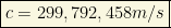
although you often take it as 

and 

![\left[c\right]=LT^{-1}](https://s0.wp.com/latex.php?latex=%5Cleft%5Bc%5Cright%5D%3DLT%5E%7B-1%7D&bg=f9f7e1&fg=000000&s=0&c=20201002)
3. Planck’s constant. 

Planck’s constant (or its rationalized version), is the fundamental universal constant in Quantum Physics (Quantum Mechanics, Quantum Field Theory). It gives

Indeed, quanta are the minimal units of energy. That is, you can not divide further a quantum of light, since it is indivisible by definition! Furthermore, the de Broglie relationship relates momentum and wavelength for any particle, and it emerges from the combination of special relativity and the quantum hypothesis:
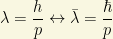
In the case of massive particles, it yields
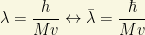
In the case of massless particles (photons, gluons, gravitons,…)


Planck’s constant also appears to be essential to the uncertainty principle of Heisenberg:
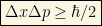

Some particularly important values of this constant are:


It is also useful to know that


or


Planck constant has dimension of 

4. Gravitational constant. 
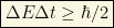
Apparently, it is not like the others but it can also define some particular scale when combined with Special Relativity. Without entering into further details (since I have not discussed General Relativity yet in this blog), we can calculate the escape velocity of a body moving at the speed of light


5. Electric fundamental charge. 
It is generally chosen as fundamental charge the electric charge of the positron (positive charged “electron”). Its value is:

where C denotes Coulomb. Of course, if you know about quarks with a fraction of this charge, you could ask why we prefer this one. Really, it is only a question of hystory of Science, since electrons were discovered first (and positrons). Quarks, with one third or two thirds of this amount of elementary charge, were discovered later, but you could define the fundamental unit of charge as multiple or entire fraction of this charge. Moreover, as far as we know, electrons are “elementary”/”fundamental” entities, so, we can use this charge as unit and we can define quark charges in terms of it too. Electric charge is not a fundamental unit in the SI system of units. Charge flow, or electric current, is.
An amazing property of the above 5 constants is that they are “universal”. And, for instance, energy is related with other magnitudes in theories where the above constants are present in a really wonderful and unified manner:

Caution: k is not the Boltzmann constant but the wave number.
There is a sixth “fundamental” constant related to electromagnetism, but it is also related to the speed of light, the electric charge and the Planck’s constant in a very sutble way. Let me introduce you it too…
6. Coulomb constant. 
This is a second constant related to classical electromagnetism, like the speed of light in vacuum. Coulomb’s constant, the electric force constant, or the electrostatic constant (denoted

Its experimental value is

Generally, the Coulomb constant is dropped out and it is usually preferred to express everything using the electric permitivity of vacuum 

H.E.P. units
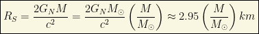
High Energy Physicists use to employ units in which the velocity is measured in fractions of the speed of light in vacuum, and the action/angular momentum is some multiple of the Planck’s constant. These conditions are equivalent to set


Complementarily, or not, depending on your tastes and preferences, you can also set the Boltzmann’s constant to the unit as well

and thus the complete HEP system is defined if you set
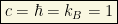
This “natural” system of units is lacking yet a scale of energy. Then, it is generally added the electron-volt 
This system of units have remarkable conversion factors
A) 
B) 
C)

D)
E) 
F)

This system of units, therefore, leaves free only the energy scale (generally it is chosen the electron-volt) and the electric measure of fundamentl charge. Every other unit can be related to energy/charge. It is truly remarkable than doing this (turning invisible the above three constants) you can “unify” different magnitudes due to the fact these conventions make them equivalent. For instance, with natural units:
1) Length=Time=1/Energy=1/Mass.
It is due to 


Note that natural units turn invisible the units we set to the unit! That is the key of the procedure. It simplifies equations and expressions. Of course, you must be careful when you reintroduce constants!
2) Energy=Mass=Momemntum=Temperature.
It is due to 

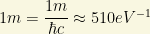
One extra bonus for theoretical physicists is that natural units allow to build and write proper lagrangians and hamiltonians (certain mathematical operators containing the dynamics of the system enconded in them), or equivalently the action functional, with only the energy or “mass” dimension as “free parameter”. Let me show how it works.
Natural units in HEP identify length and time dimensions. Thus ![\left[L\right]=\left[T\right]](https://s0.wp.com/latex.php?latex=%5Cleft%5BL%5Cright%5D%3D%5Cleft%5BT%5Cright%5D&bg=f9f7e1&fg=000000&s=0&c=20201002)
![\boxed{\left[L\right]=\left[T\right]=\left[E\right]^{-1}}](https://s0.wp.com/latex.php?latex=%5Cboxed%7B%5Cleft%5BL%5Cright%5D%3D%5Cleft%5BT%5Cright%5D%3D%5Cleft%5BE%5Cright%5D%5E%7B-1%7D%7D&bg=f9f7e1&fg=000000&s=0&c=20201002)
The speed of light identifies energy and mass, and thus, we can often heard about “mass-dimension” of a lagrangian in the following sense. HEP units can be thought as defining “everything” in terms of energy, from the pure dimensional ground. That is, every physical dimension is (in HEP units) defined by a power of energy:
![\boxed{\left[E\right]^n}](https://s0.wp.com/latex.php?latex=%5Cboxed%7B%5Cleft%5BE%5Cright%5D%5En%7D&bg=f9f7e1&fg=000000&s=0&c=20201002)
Thus, we can refer to any magnitude simply saying the power of such physical dimension (or you can think logarithmically to understand it easier if you wish). With this convention, and recalling that energy dimension is mass dimension, we have that
![\left[L\right]=\left[T\right]=-1](https://s0.wp.com/latex.php?latex=%5Cleft%5BL%5Cright%5D%3D%5Cleft%5BT%5Cright%5D%3D-1&bg=f9f7e1&fg=000000&s=0&c=20201002)
![\left[E\right]=\left[M\right]=1](https://s0.wp.com/latex.php?latex=%5Cleft%5BE%5Cright%5D%3D%5Cleft%5BM%5Cright%5D%3D1&bg=f9f7e1&fg=000000&s=0&c=20201002)
Using these arguments, the action functional is a pure dimensionless quantity, and thus, in D=4 spacetime dimensions, lagrangian densities must have dimension 4 ( or dimension D is a general spacetime).
![\displaystyle{S=\int d^4x \mathcal{L}\rightarrow \left[\mathcal{L}\right]=4}](https://s0.wp.com/latex.php?latex=%5Cdisplaystyle%7BS%3D%5Cint+d%5E4x+%5Cmathcal%7BL%7D%5Crightarrow+%5Cleft%5B%5Cmathcal%7BL%7D%5Cright%5D%3D4%7D&bg=f9f7e1&fg=000000&s=0&c=20201002)
![\displaystyle{S=\int d^Dx \mathcal{L}\rightarrow \left[\mathcal{L}\right]=D}](https://s0.wp.com/latex.php?latex=%5Cdisplaystyle%7BS%3D%5Cint+d%5EDx+%5Cmathcal%7BL%7D%5Crightarrow+%5Cleft%5B%5Cmathcal%7BL%7D%5Cright%5D%3DD%7D&bg=f9f7e1&fg=000000&s=0&c=20201002)
In D=4 spacetime dimensions, it can be easily showed that
![\left[\partial_\mu\right]=\left[\Phi\right]=\left[A^\mu\right]=1](https://s0.wp.com/latex.php?latex=%5Cleft%5B%5Cpartial_%5Cmu%5Cright%5D%3D%5Cleft%5B%5CPhi%5Cright%5D%3D%5Cleft%5BA%5E%5Cmu%5Cright%5D%3D1&bg=f9f7e1&fg=000000&s=0&c=20201002)
![\left[\Psi_D\right]=\left[\Psi_M\right]=\left[\chi\right]=\left[\eta\right]=\dfrac{3}{2}](https://s0.wp.com/latex.php?latex=%5Cleft%5B%5CPsi_D%5Cright%5D%3D%5Cleft%5B%5CPsi_M%5Cright%5D%3D%5Cleft%5B%5Cchi%5Cright%5D%3D%5Cleft%5B%5Ceta%5Cright%5D%3D%5Cdfrac%7B3%7D%7B2%7D&bg=f9f7e1&fg=000000&s=0&c=20201002)
where 


![\boxed{\left[\Phi\right]=\left[A_\mu\right]=\dfrac{D-2}{2}\equiv E^{\frac{D-2}{2}}=M^{\frac{D-2}{2}}}](https://s0.wp.com/latex.php?latex=%5Cboxed%7B%5Cleft%5B%5CPhi%5Cright%5D%3D%5Cleft%5BA_%5Cmu%5Cright%5D%3D%5Cdfrac%7BD-2%7D%7B2%7D%5Cequiv+E%5E%7B%5Cfrac%7BD-2%7D%7B2%7D%7D%3DM%5E%7B%5Cfrac%7BD-2%7D%7B2%7D%7D%7D&bg=f9f7e1&fg=000000&s=0&c=20201002)
![\boxed{\left[\Psi\right]=\dfrac{D-1}{2}\equiv E^{\frac{D-1}{2}}=M^{\frac{D-1}{2}}}](https://s0.wp.com/latex.php?latex=%5Cboxed%7B%5Cleft%5B%5CPsi%5Cright%5D%3D%5Cdfrac%7BD-1%7D%7B2%7D%5Cequiv+E%5E%7B%5Cfrac%7BD-1%7D%7B2%7D%7D%3DM%5E%7B%5Cfrac%7BD-1%7D%7B2%7D%7D%7D&bg=f9f7e1&fg=000000&s=0&c=20201002)
Remark (for QFT experts only): Don’t confuse mass dimension with the final transverse polarization degrees or “degrees of freedom” of a particular field, i.e., “components” minus “gauge constraints”. E.g.: a gauge vector field has 
In summary:
i) HEP units are based on QM (Quantum Mechanics), SR (Special Relativity) and Statistical Mechanics (Entropy and Thermodynamics).
ii) HEP units need to introduce a free energy scale, and it generally drives us to use the eV or electron-volt as auxiliary energy scale.
iii) HEP units are useful to dimensional analysis of lagrangians (and hamiltonians) up to “mass dimension”.
Stoney Units
In Physics, the Stoney units form a alternative set of natural units named after the Irish physicist George Johnstone Stoney, who first introduced them as we know it today in 1881. However, he presented the idea in a lecture entitled “On the Physical Units of Nature” delivered to the British Association before that date, in 1874. They are the first historical example of natural units and “unification scale” somehow. Stoney units are rarely used in modern physics for calculations, but they are of historical interest but some people like Wilczek has written about them (see, e.g., http://arxiv.org/abs/0708.4361). These units of measurement were designed so that certain fundamental physical constants are taken as reference basis without the Planck scale being explicit, quite a remarkable fact! The set of constants that Stoney used as base units is the following:
A) Electric charge, 
B) Speed of light in vacuum, 
C) Gravitational constant, 
D) The Reciprocal of Coulomb constant, 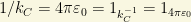
Stony units are built when you set these four constants to the unit, i.e., equivalently, the Stoney System of Units (S) is determined by the assignments:
Interestingly, in this system of units, the Planck constant is not equal to the unit and it is not “fundamental” (Wilczek remarked this fact here ) but:

Today, Planck units are more popular Planck than Stoney units in modern physics, and even there are many physicists who don’t know about the Stoney Units! In fact, Stoney was one of the first scientists to understand that electric charge was quantized!; from this quantization he deduced the units that are now named after him.
The Stoney length and the Stoney energy are collectively called the Stoney scale, and they are not far from the Planck length and the Planck energy, the Planck scale. The Stoney scale and the Planck scale are the length and energy scales at which quantum processes and gravity occur together. At these scales, a unified theory of physics is thus likely required. The only notable attempt to construct such a theory from the Stoney scale was that of H. Weyl, who associated a gravitational unit of charge with the Stoney length and who appears to have inspired Dirac’s fascination with the large number hypothesis. Since then, the Stoney scale has been largely neglected in the development of modern physics, although it is occasionally discussed to this day. Wilczek likes to point out that, in Stoney Units, QM would be an emergent phenomenon/theory, since the Planck constant wouldn’t be present directly but as a combination of different constants. By the other hand, the Planck scale is valid for all known interactions, and does not give prominence to the electromagnetic interaction, as the Stoney scale does. That is, in Stoney Units, both gravitation and electromagnetism are on equal footing, unlike the Planck units, where only the speed of light is used and there is no more connections to electromagnetism, at least, in a clean way like the Stoney Units do. Be aware, sometimes, rarely though, Planck units are referred to as Planck-Stoney units.
What are the most interesting Stoney system values? Here you are the most remarkable results:
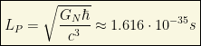
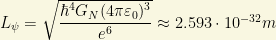
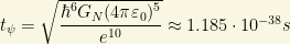
1) Stoney Length, 

2) Stoney Mass, 

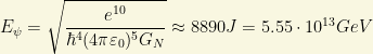
3) Stoney Energy, 

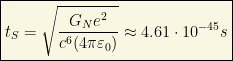
4) Stoney Time, 
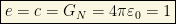
5) Stoney Charge, 

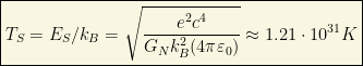
6) Stoney Temperature, 
Planck Units
The reference constants to this natural system of units (generally denoted by P) are the following 4 constants:
1) Gravitational constant.
2) Speed of light.
3) Planck constant or rationalized Planck constant.
4) Boltzmann constant.
The Planck units are got when you set these 4 constants to the unit, i.e.,

It is often said that Planck units are a system of natural units that is not defined in terms of properties of any prototype, physical object, or even features of any fundamental particle. They only refer to the basic structure of the laws of physics: c and G are part of the structure of classical spacetime in the relativistic theory of gravitation, also known as general relativity, and ℏ captures the relationship between energy and frequency which is at the foundation of elementary quantum mechanics. This is the reason why Planck units particularly useful and common in theories of quantum gravity, including string theory or loop quantum gravity.
This system defines some limit magnitudes, as follows:
1) Planck Length, 
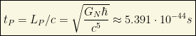
2) Planck Time, 
3) Planck Mass, 

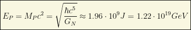
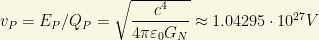
4) Planck Energy, 
5) Planck charge, 
In Lorentz-Heaviside electromagnetic units

In Gaussian electromagnetic units

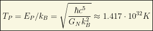
6) Planck temperature, 
From these “fundamental” magnitudes we can build many derived quantities in the Planck System:
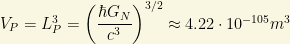
1) Planck area.
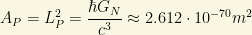
2) Planck volume.
3) Planck momentum.

A relatively “small” momentum!
4) Planck force.
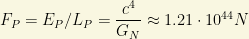
It is independent from Planck constant! Moreover, the Planck acceleration is

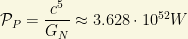
5) Planck Power.
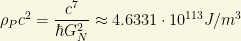
6) Planck density.
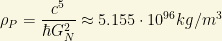
Planck density energy would be equal to
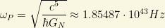
7) Planck angular frequency.
8) Planck pressure.

Note that Planck pressure IS the Planck density energy!
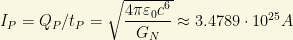
9) Planck current.
10) Planck voltage.
11) Planck impedance.
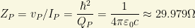
A relatively small impedance!
12) Planck capacitor.

Interestingly, it depends on the gravitational constant!
Some Planck units are suitable for measuring quantities that are familiar from daily experience. In particular:
1 Planck mass is about 22 micrograms.
1 Planck momentum is about 6.5 kg m/s
1 Planck energy is about 500kWh.
1 Planck charge is about 11 elementary (electronic) charges.
1 Planck impendance is almost 30 ohms.
Moreover:
i) A speed of 1 Planck length per Planck time is the speed of light, the maximum possible speed in special relativity.
ii) To understand the Planck Era and “before” (if it has sense), supposing QM holds yet there, we need a quantum theory of gravity to be available there. There is no such a theory though, right now. Therefore, we have to wait if these ideas are right or not.
iii) It is believed that at Planck temperature, the whole symmetry of the Universe was “perfect” in the sense the four fundamental foces were “unified” somehow. We have only some vague notios about how that theory of everything (TOE) would be.
The physical dimensions of the known Universe in terms of Planck units are “dramatic”:
i) Age of the Universe is about 
ii) Diameter of the observable Universe is about

iii) Current temperature of the Universe is about

iv) The observed cosmological constant is about

v) The mass of the Universe is about 
vi) The Hubble constant is

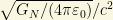
Schrödinger Units
The Schrödinger Units do not obviously contain the term c, the speed of light in a vacuum. However, within the term of the Permittivity of Free Space [i.e., electric constant or vacuum permittivity], and the speed of light plays a part in that particular computation. The vacuum permittivity results from the reciprocal of the speed of light squared times the magnetic constant. So, even though the speed of light is not apparent in the Schrödinger equations it does exist buried within its terms and therefore influences the decimal placement issue within square roots. The essence of Schrödinger units are the following constants:
A) Gravitational constant
B) Planck constant
C) Boltzmann constant
D) Coulomb constant or equivalently the electric permitivity of free space/vacuum 
E) The electric charge of the positron
In this sistem 
1) Schrödinger Length 
2) Schrödinger time 
3) Schrödinger mass 

4) Schrödinger energy 
5) Schrödinger charge 
6) Schrödinger temperature 

Atomic Units
There are two alternative systems of atomic units, closely related:
1) Hartree atomic units:

2) Rydberg atomic units:


There, 

The units are adapted to characterize the behavior of an electron in the ground state of a hydrogen atom. For example, using the Hartree convention, in the Böhr model of the hydrogen atom, an electron in the ground state has orbital velocity = 1, orbital radius = 1, angular momentum = 1, ionization energy equal to 1/2, and so on.
Some quantities in the Hartree system of units are:
1) Atomic Length (also called Böhr radius):
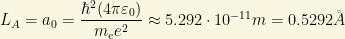
2) Atomic Time:
3) Atomic Mass:

4) Atomic Energy:

5) Atomic electric Charge:

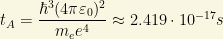
6) Atomic temperature:
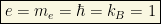
The fundamental unit of energy is called the Hartree energy in the Hartree system and the Rydberg energy in the Rydberg system. They differ by a factor of 2. The speed of light is relatively large in atomic units (137 in Hartree or 274 in Rydberg), which comes from the fact that an electron in hydrogen tends to move much slower than the speed of light. The gravitational constant is extremely small in atomic units (about 10−45), which comes from the fact that the gravitational force between two electrons is far weaker than the Coulomb force . The unit length, LA, is the so-called and well known Böhr radius, a0.
The values of c and e shown above imply that 
QCD Units
In the framework of Quantum Chromodynamics, a quantum field theory (QFT) we know as QCD, we can define the QCD system of units based on:
1) QCD Length 

and where 
2) QCD Time 
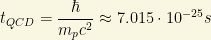
3) QCD Mass 

4) QCD Energy 

Thus, QCD energy is about 1 GeV!
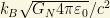
5) QCD Temperature 

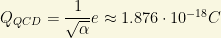
6) QCD Charge 
In Heaviside-Lorent units:

In Gaussian units:
Geometrized Units
The geometrized unit system, used in general relativity, is not a completely defined system. In this system, the base physical units are chosen so that the speed of light and the gravitational constant are set equal to unity. Other units may be treated however desired. By normalizing appropriate other units, geometrized units become identical to Planck units. That is, we set:

and the remaining constants are set to the unit according to your needs and tastes.
Conversion Factors
This table from wikipedia is very useful:

where:
i)
ii) 
Some conversion factors for geometrized units are also available:
Conversion from kg, s, C, K into m:


Conversion from m, s, C, K into kg:


Conversion from m, kg, C, K into s


Conversion from m, kg, s, K into C


Conversion from m, kg, s, C into K


Or you can read off factors from this table as well:

and

Advantages and Disadvantages of Natural Units
Natural units have some advantages (“Pro”):
1) Equations and mathematical expressions are simpler in Natural Units.
2) Natural units allow for the match between apparently different physical magnitudes.
3) Some natural units are independent from “prototypes” or “external patterns” beyond some clever and trivial conventions.
4) They can help to unify different physical concetps.
However, natural units have also some disadvantages (“Cons”):
1) They generally provide less precise measurements or quantities.
2) They can be ill-defined/redundant and own some ambiguity. It is also caused by the fact that some natural units differ by numerical factors of pi and/or pure numbers, so they can not help us to understand the origin of some pure numbers (adimensional prefactors) in general.
Moreover, you must not forget that natural units are “human” in the sense you can addapt them to your own needs, and indeed,you can create your own particular system of natural units! However, said this, you can understand the main key point: fundamental theories are who finally hint what “numbers”/”magnitudes” determine a system of “natural units”.
Remark: the smart designer of a system of natural unit systems must choose a few of these constants to normalize (set equal to 1). It is not possible to normalize just any set of constants. For example, the mass of a proton and the mass of an electron cannot both be normalized: if the mass of an electron is defined to be 1, then the mass of a proton has to be 

where
Fritzsch-Xing plot
Fritzsch and Xing have developed a very beautiful plot of the fundamental constants in Nature (those coming from gravitation and the Standard Model). I can not avoid to include it here in the 2 versions I have seen it. The first one is “serious”, with 29 “fundamental constants”:

However, I prefer the “fun version” of this plot. This second version is very cool and it includes 28 “fundamental constants”:

The Okun Cube
Long ago, L.B. Okun provided a very interesting way to think about the Planck units and their meaning, at least from current knowledge of physics! He imagined a cube in 3d in which we have 3 different axis. Planck units are defined as we have seen above by 3 constants 

Or equivalently, sometimes it is seen as an equivalent sketch ( note the Planck constant is NOT rationalized in the next cube, but it does not matter for this graphical representation):

Classical physics (CP) corresponds to the vanishing of the 3 constants, i.e., to the origin 
Newtonian mechanics (NM) , or more precisely newtonian gravity plus classical mechanics, corresponds to the “point” 
Special relativity (SR) corresponds to the point 
Quantum mechanics (QM) corresponds to the point 
Quantum Field Theory (QFT) corresponds to the point 
Quantum Gravity (QG) would correspond to the point 
Finally, the Theory Of Everything (TOE) would be the theory in the last free corner, that arising in the vertex 
Some final remarks and questions
1) Are fundamental “constants” really constant? Do they vary with energy or time?
2) How many fundamental constants are there? This questions has provided lots of discussions. One of the most famous was this one:
http://arxiv.org/abs/physics/0110060
The trialogue (or dialogue if you are precise with words) above discussed the opinions by 3 eminent physicists about the number of fundamental constants: Michael Duff suggested zero, Gabriel Veneziano argued that there are only 2 fundamental constants while L.B. Okun defended there are 3 fundamental constants
3) Should the cosmological constant be included as a new fundamental constant? The cosmological constant behaves as a constant from current cosmological measurements and cosmological data fits, but is it truly constant? It seems to be…But we are not sure. Quintessence models (some of them related to inflationary Universes) suggest that it could vary on cosmological scales very slowly. However, the data strongly suggest that

It is simple, but it is not understood the ultimate nature of such a “fluid” because we don’t know what kind of “stuff” (either particles or fields) can make the cosmological constant be so tiny and so abundant (about the 72% of the Universe is “dark energy”/cosmological constant) as it seems to be. We do know it can not be “known particles”. Dark energy behaves as a repulsive force, some kind of pressure/antigravitation on cosmological scales. We suspect it could be some kind of scalar field but there are many other alternatives that “mimic” a cosmological constant. If we identify the cosmological constant with the vacuum energy we obtain about 122 orders of magnitude of mismatch between theory and observations. A really bad “prediction”, one of the worst predictions in the history of physics!
Be natural and stay tuned!
LOG#041. Muons and relativity.
Posted: 2012/10/12 Filed under: Physmatics, Relativity | Tags: cosmic rays, Minkovski spacetime, muons, Physics, Physmatics, reality, Relativity, science, spacetime, special relativity, time dilation 1 Comment

QUESTION: Is the time dilation real or is it an artifact of our current theories?
There are solid arguments why time dilation is not an apparent effect but a macroscopic measurable effect. Today, we are going to discuss the “reality” of time dilation with a well known result:
Muon detection experiments!
Muons are enigmatic elementary particles from the second generation of the Standard Model with the following properties:
1st. They are created in upper atmosphere at altitudes of about 9000 m, when cosmic rays hit the Earth and they are a common secondary product in the showers created by those mysterious yet cosmic rays.
2nd. The average life span is
3rd. Typical speed is 0.998c or very close to the speed of light.
So we would expect that they could only travel at most
However, surprisingly at first sight, they can be observed at ground level! SR provides a beautiful explanation of this fact. In the rest frame S of the Earth, the lifespan of a traveling muon experiences time dilation. Let us define


A) t= half-life of muon with respect to Earth.
B) t’=half-life of muon of the moving muon (in his rest frame S’ in motion with respect to Earth).
C) According to SR, the time dilation means that 
A typical dilation factor 


If the gamma factor is bigger, the distance d’ grows and so, we can detect muons on the ground, as we do observe indeed!
Remark: In the traveling muon’s reference frame, it is at rest and the Earth is rushing up to meet it at 0.998c. The distance between it and the Earth thus is shorter than 9000m by length contraction. With respect to the muon, this distance is therefore 9000m/15 = 600m.
An alternative calculation, with approximate numbers:
Suppose muons decay into other particles with half-life of about 0.000001sec. Cosmic ray muons have speed now about v = 0.99995 c.
Without special relativity, muon would travel

Few would reach earth’s surface in that case. It we use special relativity, then plugging the corresponding gamma for 


Conclusion: a lot of muons reach the earth’s surface. And we can detect them! For instance, with the detectors on colliders, the cosmic rays detectors, and some other simpler tools.
LOG#034. Stellar aberration.
Posted: 2012/10/07 Filed under: Physmatics, Relativity | Tags: aberration formula, astronomy, electromagnetism, Relativity, spacetime, special relativity Leave a comment
In this entry, we are going to study a relativistic effect known as “stellar aberration”.
From the known Lorentz transformations of velocities (inverse case), we get:


The classical result (galilean addition of velocities) is recovered in the limit of low velocities 


Let us define


Thus, we get the component decomposition into the xy and x’y’ planes:


From this equations, we get

If


and then


From the last equation, we get

From this equation, if 


By these formaulae, the angle of a light beam propagating in space depends on the velocity of the source respect to the observer. We can observe this relativistic effect every night (supposing a good approximation that Earth’s velocity is non-relativistic, as it shows). The physical interpretation of the above aberration formulae (for the stars we watch during a skynight) is as follows: due to the Earth’s motion, a star in the zenith is seen under an angle 
Other important consequence from the stellar aberration is when we track ultra-relativistic particles (


LOG#033. Electromagnetism in SR.
Posted: 2012/10/07 Filed under: Physmatics, Relativity | Tags: electric charge, electromagnetic current, electromagnetic field, field strength, gauge theory, gauge transformations, light intensity, Lorentz force, Maxwell equations, Physmatics, Poynting vector, Relativity, spacetime, U(1), vector potential, wave number vector Leave a comment The Maxwell’s equations and the electromagnetism phenomena are one of the highest achievements and discoveries of the human kind. Thanks to it, we had radio waves, microwaves, electricity, the telephone, the telegraph, TV, electronics, computers, cell-phones, and internet. Electromagnetic waves are everywhere and everytime (as far as we know, with the permission of the dark matter and dark energy problems of Cosmology). Would you survive without electricity today?
The language used in the formulation of Maxwell equations has changed a lot since Maxwell treatise on Electromagnetis, in which he used the quaternions. You can see the evolution of the Mawell equations “portrait” with the above picture. Today, from the mid 20th centure, we can write Maxwell equations into a two single equations. However, it is less know that Maxwell equations can be written as a single equation 

Before entering into the details of electromagnetic fields, let me give some easy notions of tensor calculus. If 


Then:
![e_\mu=\Lambda^{\mu'}_{\;\; \mu} e_{\mu'}\rightarrow e_{\mu'}=\left(\Lambda^{-1}\right)_{\;\; \mu'}^{\mu}e_\mu=\left[\left(\Lambda^{-1}\right)^T\right]^{\;\; \mu}_{\nu}e_\mu](https://s0.wp.com/latex.php?latex=e_%5Cmu%3D%5CLambda%5E%7B%5Cmu%27%7D_%7B%5C%3B%5C%3B+%5Cmu%7D+e_%7B%5Cmu%27%7D%5Crightarrow+e_%7B%5Cmu%27%7D%3D%5Cleft%28%5CLambda%5E%7B-1%7D%5Cright%29_%7B%5C%3B%5C%3B+%5Cmu%27%7D%5E%7B%5Cmu%7De_%5Cmu%3D%5Cleft%5B%5Cleft%28%5CLambda%5E%7B-1%7D%5Cright%29%5ET%5Cright%5D%5E%7B%5C%3B%5C%3B+%5Cmu%7D_%7B%5Cnu%7De_%5Cmu&bg=f9f7e1&fg=000000&s=0&c=20201002)
Note, we have used with caution:
1st. Einstein’s convention: sum over repeated subindices and superindices is understood, unless it is stated some exception.
2nd. Free indices can be labelled to the taste of the user segment.
3rd. Careful matrix type manipulations.
We define a contravariant vector (or tensor (1,0) ) as some object transforming in the next way:

where 
In similar way, we can define a covariant vector ( or tensor (0,1) ) with the aid of the following equations
![\boxed{a_{\mu'}=\left[\left(\Lambda^{-1}\right)^{T}\right]_{\mu'}^{\:\;\; \nu}a_\nu}\leftrightarrow\boxed{a_{\mu'}=\left(\dfrac{\partial x^{\nu}}{\partial x^{\mu'}}\right)a_\nu}](https://s0.wp.com/latex.php?latex=%5Cboxed%7Ba_%7B%5Cmu%27%7D%3D%5Cleft%5B%5Cleft%28%5CLambda%5E%7B-1%7D%5Cright%29%5E%7BT%7D%5Cright%5D_%7B%5Cmu%27%7D%5E%7B%5C%3A%5C%3B%5C%3B+%5Cnu%7Da_%5Cnu%7D%5Cleftrightarrow%5Cboxed%7Ba_%7B%5Cmu%27%7D%3D%5Cleft%28%5Cdfrac%7B%5Cpartial+x%5E%7B%5Cnu%7D%7D%7B%5Cpartial+x%5E%7B%5Cmu%27%7D%7D%5Cright%29a_%5Cnu%7D&bg=f9f7e1&fg=000000&s=0&c=20201002)
Note:

Contravariant tensors of second order ( tensors type (2,0)) are defined with the next equations:

Covariant tensors of second order ( tensors type (0,2)) are defined similarly:

Mixed tensors of second order (tensors type (1,1)) can be also made:

We can summarize these transformations rules in matrix notation making the transcript from the index notation easily:
1st. Contravariant vectors change of coordinates rule:

2nd. Covariant vectors change of coordinates rule:

3rd. (2,0)-tensors change of coordinates rule:

4rd. (0,2)-tensors change of coordinates rule:

5th. (1,1)-tensors change of coordinates rule:

Indeed, without taking care with subindices and superindices, and the issue of the inverse and transpose for transformation matrices, a general tensor type (r,s) is defined as follows:

We return to electromagnetism! The easiest examples of electromagnetic wave motion are plane waves:

where

Indeed, the cuadrivector K can be “guessed” from the phase invariant (

where 

and so

Now, let me discuss different notions of velocity when we are considering electromagnetic fields, beyond the usual notions of particle velocity and observer relative motion, we have the following notions of velocity in relativistic electromagnetism:
1st. The light speed c. It is the ultimate limit in vacuum and SR to the propagation of electromagnetic signals. Therefore, it is sometimes called energy transfer velocity in vacuum or vacuum speed of light.
2nd. Phase velocity 


From the definition of cuadrivector wave length, we deduce:

Then, we can rewrite the distinguish three cases according to the sign of the invariant 
a) 

b)

c)

3rd. Group velocity 

where we used the Planck relationships for photons 


4th. Particle velocity. It is defined in SR by the cuadrivector

5th. Observer relative velocity, V. It is the velocity (constant) at which two inertial observes move.
There is a nice relationship between the group velocity, the phase velocity and the energy transfer, the lightspeed in vacuum. To see it, look at the invariant:

Deriving this expression, we get

so we have the very important equation

Other important concept in electromagnetism is “light intensity”. Light intensity can be thought like the “flux of light”, and you can imagine it both in the wave or particle (photon corpuscles) theory in a similar fashion. Mathematically speaking:

so 


The relativistic momentum can be related to the wavelength cuadrivector using the Planck relation 


and then

In matrix notation, the whole change is written as:

so

Using the first two equations, we get:

Using the first and the third equation, we obtain:

Dividing the last two equations, we deduce:

This formula is the so-called stellar aberration formula, and we will dedicate it a post in the future.
If we write the first equation with the aid of frequency f (and 

where we wrote the frequency of the source as 

Now, we are going to introduce a very important object in electromagnetism: the electric charge and the electric current. We are going to make an analogy with the momenergy 

where 


and


We conclude:
1st. Length contraction implies that the charge density increases by a gamma factor, i.e., 
2nd. The crystal lattice “hole” velocity 

3rd. The existence of charges in motion when seen from an inertial frame (boosted from a rest reference S) implies that in a moving reference frame electric fields are not alone but with magnetic fields. From this perspective, magnetic fields are associated to the existence of moving charges. That is, electric fields and magnetic fields are intimately connected and they are caused by static and moving charges, as we do know from classical non-relativistic physics.
Remember now the general expression of the FORPOWER tetravector, or Power-Force tetravector, in SR:

and using the metric, with the mainly plus convention, we get the covariant componets for the power-force tetravector:

We define the Lorentz force as the sum of the electric and magnetic forces

Noting that 

And now, we realize that we can understand the electromagnetic force in terms of a tensor (1,1), i.e., a matrix, if we write:

so

Therefore,

where the components of the (1,1) tensor can be read:

We can lower the indices with the metric 


with

Similarly

Please, note that 


From this equation we deduce that:

Example: In the S-frame we have the fields 


Surprinsingly, or not, the S’-observer sees a boosted electric field (non null!), a boosted magnetic field, a boosted non-null Coulomb force and a null Lorentz force!
We can generalize the above transformations to the case of a general velocity in 3d-space


![\mathbf{E}_{\perp'}=\gamma \left[\mathbf{E}_\perp+(\mathbf{v}\times \mathbf{B})_\perp\right]=\gamma \left[\mathbf{E}_\perp+(\mathbf{v}\times \mathbf{B})\right]](https://s0.wp.com/latex.php?latex=%5Cmathbf%7BE%7D_%7B%5Cperp%27%7D%3D%5Cgamma+%5Cleft%5B%5Cmathbf%7BE%7D_%5Cperp%2B%28%5Cmathbf%7Bv%7D%5Ctimes+%5Cmathbf%7BB%7D%29_%5Cperp%5Cright%5D%3D%5Cgamma+%5Cleft%5B%5Cmathbf%7BE%7D_%5Cperp%2B%28%5Cmathbf%7Bv%7D%5Ctimes+%5Cmathbf%7BB%7D%29%5Cright%5D&bg=f9f7e1&fg=000000&s=0&c=20201002)
![\mathbf{B}_{\perp'}=\gamma \left[\mathbf{B}_\perp-\dfrac{1}{c^2}(\mathbf{v}\times \mathbf{E})_\perp\right]=\gamma \left[\mathbf{B}_\perp-\dfrac{1}{c^2}(\mathbf{v}\times \mathbf{E})\right]](https://s0.wp.com/latex.php?latex=%5Cmathbf%7BB%7D_%7B%5Cperp%27%7D%3D%5Cgamma+%5Cleft%5B%5Cmathbf%7BB%7D_%5Cperp-%5Cdfrac%7B1%7D%7Bc%5E2%7D%28%5Cmathbf%7Bv%7D%5Ctimes+%5Cmathbf%7BE%7D%29_%5Cperp%5Cright%5D%3D%5Cgamma+%5Cleft%5B%5Cmathbf%7BB%7D_%5Cperp-%5Cdfrac%7B1%7D%7Bc%5E2%7D%28%5Cmathbf%7Bv%7D%5Ctimes+%5Cmathbf%7BE%7D%29%5Cright%5D&bg=f9f7e1&fg=000000&s=0&c=20201002)
The last equal in the last two equations is due to the orthogonality of the position vector to the velocity in 3d space due to the cross product. From these equations, we easily obtain:


and similarly with the magnetic field. The final tranformations we obtain are:
![\boxed{E'=E_{\parallel'}+E_{\perp'}=\dfrac{(v\cdot E)v}{v^2}+\gamma \left[ E-\dfrac{(v\cdot E)v}{v^2}+v\times B\right]}](https://s0.wp.com/latex.php?latex=%5Cboxed%7BE%27%3DE_%7B%5Cparallel%27%7D%2BE_%7B%5Cperp%27%7D%3D%5Cdfrac%7B%28v%5Ccdot+E%29v%7D%7Bv%5E2%7D%2B%5Cgamma+%5Cleft%5B+E-%5Cdfrac%7B%28v%5Ccdot+E%29v%7D%7Bv%5E2%7D%2Bv%5Ctimes+B%5Cright%5D%7D&bg=f9f7e1&fg=000000&s=0&c=20201002)
![\boxed{B'=B_{\parallel'}+B_{\perp'}=\dfrac{(v\cdot B)v}{v^2}+\gamma \left[ B-\dfrac{(v\cdot B)v}{v^2}-v\times E\right]}](https://s0.wp.com/latex.php?latex=%5Cboxed%7BB%27%3DB_%7B%5Cparallel%27%7D%2BB_%7B%5Cperp%27%7D%3D%5Cdfrac%7B%28v%5Ccdot+B%29v%7D%7Bv%5E2%7D%2B%5Cgamma+%5Cleft%5B+B-%5Cdfrac%7B%28v%5Ccdot+B%29v%7D%7Bv%5E2%7D-v%5Ctimes+E%5Cright%5D%7D&bg=f9f7e1&fg=000000&s=0&c=20201002)
Equivalently


In the limit where 


There are two invariants for electromagnetic fields:


It can be checked that

and


and where we have defined the dual electromagnetic field as

or if we write it in components ( duality sends 


We can guess some consequences for the electromagnetic invariants:
1st. If 


2nd. As 


3rd. If E=cB, i.e., if 
4th. If there is a electric field but there is no magnetic field B in S, a Lorentz transformation to a pure B’ in S’ is impossible and viceversa.
5th. If the electric field is such that 

6th. There is a trick to remember the two invariants. It is due to Riemann. We can build the hexadimensional vector( six-vector, or sixtor) and complex valued entity

The two invariants are easily obtained squaring F:

We can introduce now a vector potencial tetravector:

This tetravector is also called gauge field. We can write the Maxwell tensor in terms of this field:

It can be easily probed that, up to a multiplicative constant in front of the electric current tetravector, the first set of Maxwell equations are:

The second set of Maxwell equations (sometimes called Bianchi identities) can be written as follows:

The Maxwell equations are invariant under the gauge transformations in spacetime:

where the potential tetravector and the function 
Some elections of gauge are common in the solution of electromagnetic problems:
A) Lorentz gauge:

B) Coulomb gauge:

C) Temporal gauge:

If we use the Lorentz gauge, and the Maxwell equations without sources, we deduce that the vector potential components satisfy the wave equation, i.e.,

Finally, let me point out an important thing about Maxwell equations. Specifically, about its invariance group. It is known that Maxwell equations are invariant under Lorentz transformations, and it was the guide Einstein used to extend galilean relativity to the case of electromagnetic fields, enlarging the mechanical concepts. But, the larger group leaving invariant the Maxwell equation’s invariant is not the Lorentz group but the conformal group. But it is another story unrelated to this post.
LOG#032. Invariance and relativity.
Posted: 2012/09/30 Filed under: Physmatics, Relativity | Tags: contravariant, covariant, Levi-Civita tensor., lightlike, metric, Physmatics, Relativity, spacelike, spacetime, tensors, timelike, vectors Leave a comment
Invariance, symmetry and invariant quantities are in the essence, heart and core of Physmatics. Let me begin this post with classical physics. Newton’s fundamental law reads:

Suppose two different frames obtained by a pure translation in space:

or

We select to make things simpler

We can easily observe by direct differentiation that Newton’s fundamental is invariant under translations in space, since mere substitution provides:

since

By the other hand, rotations around a fixed axis, say the z-axis, are transformations given by:

If we multiply by the mass these last equations and we differentiate with respect to time twice, keeping constant 


or

Thus, we can say that Newton’s fundamental law is invariant under spatial translations and rotations. Its form is kept constant under those kind of transformations. Generally speaking, we also say that Newton’s law is “covariant”, but nowadays it is an abuse of language since the word covariant means something different in tensor analysis. So, be aware about the word “covariant” (specially in old texts). Today, we talk about “invariant laws”, or about the symmetry of certain equations under certain set of (group) transformations.
Newton’s law use the concept of acceleration:

with


or, in compact form

And then, the following equations are invariant under translations in space and rotations:


Intrinsic components of the aceleration provide a decomposition

where we define

where 

In the case of motion along a general curve, we can approximate the motion in every point of the curve by a circle of radius R, and thus

By the other hand,

and we get the known expression for the centripetal acceleration:

More about invariant quantities in Classical Physics: the scalar (sometimes called dot) product of two vectors is invariant, since the length of every vector is constant in euclidean spaces under rotations and translations. For instance,

In matrix form,

where we have introduced the 

The scalar (dot) product can be computed with any vector quantity:

Moreover, there is a coordinate free definition as well:

Note that the invariance of the dot product implies the invariance of classical kinetic energy, since:

We have also the important invariant quantities:


where the second equality holds if the force is constant along the trajectory. Moreover, in relativistic electromagnetism, you also get the wave-number 4-vector:

and the invariant 

where the phase invariant reads

Therefore, we deduce that

and the wave number vector satisfies the following relation with the wave-length

There is another important set of transformations or symmetry in classical physics. It is related to inertial frames. Galileo discovered that the laws of motion are the same for every inertial observer, i.e., the laws of Mechanics are invariant for inertial frames! A Galilean transformation is defined by:

where 

and then

And thus, the accelerations (and forces) that observe different inertial ( i.e., reference frames moving with constant relative velocity) frames are the same

And now, about symmetry. What are the symmetries of Physics? There are many interesting transformations and space-time symmetries. A non-completely exhaustive list is this one:
1. Translations in space.
2. Translations in time.
3. Rotations around some axis ( and with fixed angle).
4. Uniform velocity in straight line, a.k.a., galilean transformations for inertial observers. This symmetry “becomes” Lorentz boosts in the spacetime analogue of special relativity.
5. Time reversal ( inversion of the direction of time), T.
6. Reflections in space (under “a mirror”). It is also called parity P.
7. Matter-antimatter interchange, or charge conjugation symmetry, C.
8. Interchange of identical atoms/particles.
9. Scale transformations 
10. Conformal transformations (in the complex plane or in complex spaces).
11. Arbitrary coordinate transformations (they are also called general coordinate transformations).
12. Quantum-mechanical (gauge) phase symmetry: 
Beyon general vectors, in classical physics we also find “axial” vectors (also called “pseudovectors”). Pseudovectors or axial vectors are formed by the 3d “cross”/outer/vector product:

Some examples are the angular momentum

or the magnetic force

Interestingly, the main difference between axial and polar vectors, i.e., between common vectors and pseudovectors is the fact that under P (parity), pseudovectors are “invariant” while common vectors change their sign, i.e., polar vectors become the opposite vector under reflection, and pseudovectors remain invariant. It can be easily found by inspection in the definition of angular momentum or the magnetic force ( or even the general definition of cross product given above).
Now, we turn our attention to invariants in special relativity. I will introduce a very easy example to give a gross idea of how the generalization of “invariant theory” works as well in special relativity. From the classical definition of power:

Using the relativistic definition of 4-momentum:

where 

Therefore, inserting the relativistic expressions for energy and force into the power equation, we obtain:

Multiplying by 2M, and using the Leibniz rule for the differentiation of a product of two functions:

or equivalently

and so

Integrating this, we deduce that

If we plug

then

and thus, we have rederived the notion of “relativistic mass”

Special relativity generalizes the notion of dot product ( scalar product) to a non-euclidean (pseudoeuclidean to be more precise) geometry. The dot product in special relativity is given by:

The sign of the temporal fourth component is conventional in the sense some people uses a minus sign for the purely spatial components and a positive sign for the temporal component. Using a more advanced notation we can write the new scalar product as follows:

where the repeated dummy index implies summation over it. This convention of understanding summation over repeated indices is called Einstein’s covention and it is due to Einstein himself. Another main point about notation is that some people prefer the use of a 


In matrix form,

Important remarks:
1st. 

2nd. The square of a “spacetime” vector is its “lenght” in spacetime. It is given by:

In particular, for the position spacetime vector

3rd. Unlike the euclidean 3d space, 4d noneuclidean spacetime introduces “objects” non-null that whose “squared lenght” is equal to zero, and even weirder, objects that could provide a negative dot product!
4th. For spacetime events given by a spacetime vector 
i) Vectors with 
ii) Vectors with 
iii) Vectos with 
Thus, in the case of the spacetime (position) vector, every event can be classified into space-like, light-like (null or isotropic) and time-like types, depending on the sign of 

The minkovskian metric has a very cool feature too. Its “square” is the identity matrix. That is,

Then, the metric is its own inverse:

In components, it reads

with

and where we have introduced the Kronecker delta symbol in four dimensions in the same manner we did in the 3d space. Therefore, the Kronecker delta has only non-null components when 

Subindices are called generally “covariant” components, while superindices are called “contravariant” components. It is evident that euclidean spaces don’t distinguish between covariant and contravariant components. The metric is the gadget we use in non-euclidean metric spaces to raise and lower indices/components from tensor quantities. Tensors are multi-oriented objects. The metric itself is a second order tensor, more precisely, the metric is a second order rank 2 covariant tensor. 4-vectors are contravariant object with a single index. Upwards single-indexed tensors are contravariant vectors, downwards single-indexed tensores are covariant vectors. When a metric is introduced, there is no need to distinguish covariant and contravariant tensors, since the components can be calculated with the aid of the metric, so we speak about n-th rank tensors. Multi-indixed objects can have some features of symmetry. The metric is symmetric itself, for instance, under the interchange of subindices ( columns and rows). So, then

What kind of general objects can we use in Minkovski spacetime or even more general spaces? Firstly, we have scalar fields or functions, i.e., functions depending only on the spacetime coordinates:

Another objetct we have found are “vectors” or “oriented segments”. In 3d space, they transform as 

In 3d space, we also found pseudovectors. They are defined via the cross product, that in components read: 


The completely antisymmetric Levi-Civita symbol has some interesting identities related with the Kronecker delta. Thus, for instance, in 2d and 3d respectively:


or

We have also the useful identity:

The n-dimensional Levi-Civita symbol is defined as:

and its product in n-dimensions

or equivalently, given a nxn matrix


This last equation provides some new quantity called pseudoscalar, different from the scalar function in the sense it changes its sign under parity in 3d, while a common 3d scalar is invariant under parity! Generally speaking, determinants (pseudoscalars) in even dimensions are parity conserving, while determinants in odd dimensions don’t conserve parity.
Like the Kronecker delta, the epsilon or Levi-Civita can be generalized to 4 dimensions (or even to D-dimensions). In 4 dimensions:

In general, unlike the Kronecker deltas, the Levi-Civita epsilon symbols are not ordinary “tensors” (quantities with subindices and superindices, with some concrete properties under coordinate transformations) but more general entities called “weighted” tensors (sometimes they are also called tensorial densities). Indeed, the generalized Kronecker delta can be defined of order 2p is a type (p,p) tensor that is a completely antisymmetric in its ”p” upper indices, and also in its ”p” lower indices. This characterization defines it up to a scalar multiplier.

Using an anti-symmetrization procedure:

In terms of an pxp determinant:

Equivalently, it could be defined by induction in the following way:

and so on.


In the particular case where p=n (the dimension of the vector space), in terms of the Levi-Civita symbol:

Under a Lorentz transformation, we have ( using matrix notation) the next transformations:


so the metric itself is “invariant” under a Lorentz transformation (boost). I would like to remark that the metric can be built from the basis vectors in the following way:

For Lorentz transformations, we get that

with

Moreover, the equation 

We can fully classify the Lorentz transformations according to the sign of the determinant and the sign of the element 

For instance, let us write 5 kind of Lorentz transformations:
1) Orthogonal rotations. They are continuous (proper) Lorentz transformations with a 3×3 submatrix 

2) Boosts. They are continuous (proper) Lorentz transformations mixing spacelike and timelike coordinates. The matrix has in this case the form:

3) PT symmetry. Discrete non-proper Lorentz transformation. It “inverts” space and time coordinates in the sense 


4) Parity. Discrete non-proper Lorentz transformation. It inverts only the spacelike components of true vectors ( be aware of pseudovectors!) in the sense 

5) Time reversal, T. Discrete non-proper Lorentz transformation. It inverts the direction of time in the sense that 

Remark: If 

LOG#026. Boosts, rapidity, HEP.
Posted: 2012/09/01 Filed under: Physmatics, Relativity | Tags: hyperbolic functions, Mathematics, Physmatics, pseudorapidity, rapidity, Relativity, spacetime Leave a comment
In euclidean two dimensional space, rotations are easy to understand in terms of matrices and trigonometric functions. A plane rotation is given by:
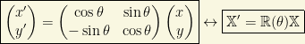
where the rotation angle is 
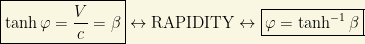
Interestingly, in minkovskian two dimensional spacetime, the analogue does exist and it is written in terms of matrices and hyperbolic trigonometric functions. A “plane” rotation in spacetime is given by:

Here, 

So, at least in the 2d spacetime case, rapidities are “additive” in the written sense.
Firstly, we are going to guess the relationship between rapidity and velocity in a single lorentzian spacetime boost. From the above equation we get:


Multiplying the first equation by 


that is

From this equation (or the boxed equations), we see that 


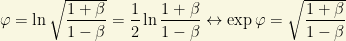
and thus


Since 

If we remember what we have learned in our previous mathematical survey, that is,

We set 
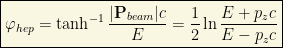
In experimental particle physics, in general 3+1 spacetime, the rapidity definition is extended as follows. Writing, from the previous equations above,
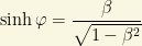
and using these two last equations, we can also write momenergy components using rapidity in the same fashion. Suppose that for some particle(objetc), its mass is 


From these equations, it is trivial to guess:

This is the completely general definition of rapidity used in High Energy Physics (HEP), with a further detail. In HEP, physicists used to select the direction of momentum in the same direction that the collision beam particles! Suppose we select some orientation, e.g.the z-axis. Then, 
In 2d spacetime, rapidities add nonlinearly according to the celebrated relativistic addition rule:
Indeed, Lorentz transformations do commute in 2d spacetime since we boost in a same direction x, we get:
with
This commutativity is lost when we go to higher dimensions. Indeed, in spacetime with more than one spatial direction that result is not true in general. If we build a Lorentz transformation with two boosts in different directions 

and it is easily checked that

Finally, there is other related quantity to rapidity that even experimentalists do prefer to rapidity. It is called: PSEUDORAPIDITY!
Pseudorapidity, often denoted by 
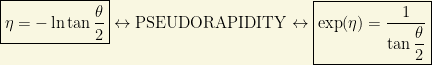
where 

The pseudorapidity in terms of the momentum is given by:

Note that, unlike rapidity, pseudorapidity depends only on the polar angle of its trajectory, and not on the energy of the particle.
In hadron collider physics, and other colliders as well, the rapidity (or pseudorapidity) is preferred over the polar angle because, loosely speaking, particle production is constant as a function of rapidity. One speaks of the “forward” direction in a collider experiment, which refers to regions of the detector that are close to the beam axis, at high pseudorapidity
The rapidity as a function of pseudorapidity is provided by the following formula:

where 
Remark: The difference in the rapidity of two particles is independent of the Lorentz boosts along the beam axis.
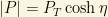
Colliders measure physical momenta in terms of transverse momentum 


Thus, we get the also useful relationship
This quantity is an observable in the collision of particles, and it can be measured as the main image of this post shows.


You must be logged in to post a comment.