
LOG#053. Derivatives of position.
Posted: 2012/11/10 Filed under: Physmatics | Tags: abseleration, absement, abserk, absition, absity, absock, absop, absounce, absrackle, absrop, acceleration, aerophone, akasha, akashaphone, calculus, classification of musical instruments, crackle, derivative, differential calculus, displacement, distance, dork, drop, dynamics, elements, farness, force, forceness, fractal, fractal calculus, geolophone, geophone, hydraulophone, infinitesimal calculus, integral, integral calculus, ionophone, jerk, jolt, jounce, Leibniz notation, loakashaphone, lock, lurch, mechanics, microphone, modern notation, momentum, motion, music, nearness, Newton notation, placement, pop, position, presackle, preseleration, presement, preserk, presity, presock, presop, presounce, presrop, shake, snap, snatch, space, speaker, speed, surge, swiftness, time, time derivatives of momentum, time derivatives of position, time integrals of momentum, time integrals of position, tug, velocity, yank 11 Comments
Position or displacement and its various derivatives define an ordered hierarchy of meaningful concepts. There are special names for the derivatives of position (first derivative is called velocity, second derivative is called acceleration, and some other derivatives with proper name), up to the eighth derivative and down to the -9th derivative (ninth integral).
We are going to study the derivatives of position and their corresponding names and special meaning in Physmatics.
0th derivative is position
In Physics, displacement or position is the vector that specifies the change in position of a point, particle, or object. The position vector directs from the reference point to the present position.
A sensor is said to be displacement-sensitive when it responds to absolute position.
For example, whereas a dynamic microphone is a velocity receiver (responds to the derivative of sound pressure or position), a carbon microphone is a displacement receiver in the sense that it responds to sound pressure or diaphragm position itself. The physical dimension of position vector or the distance is length, i.e.,
![\left[\mathbf{x}\right]=\left[ d\right]=L](https://s0.wp.com/latex.php?latex=%5Cleft%5B%5Cmathbf%7Bx%7D%5Cright%5D%3D%5Cleft%5B+d%5Cright%5D%3DL&bg=f9f7e1&fg=000000&s=0&c=20201002)
1st derivative is velocity
Velocity is defined as the rate of change of position or the rate of displacement. It is a vector physical quantity, both speed and direction are required to define it. In the SI(metric) system, it is measured in meters per second (m/s).
The scalar absolute value (magnitude) of velocity is called speed. For example, “5 metres per second” is a speed and not a vector, whereas “5 metres per second east” is a vector. The average velocity (v) of an object moving through a displacement 


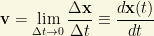
Therefore, velocity is change in position per unit of time. If the change is made “infinitesimally”, i.e., taking two very close points in time, we can define the instantanous velocity ( a.k.a, the derivative) as the limit of the average speed or two very close points when the time interval tends to zero:
Most piano-style music keyboards are approximately velocity-sensitive, within a certain specific, though limited range of key travel, i.e. to a first-order approximation, a note is made louder by hitting a key faster. Most electronic music keyboards are also velocity sensitive, and measure the time interval between switch contact closures at two different positions of key travel on each key.
The physical dimensions of velocity are
![\left[\mathbf{v}\right]=LT^{-1}](https://s0.wp.com/latex.php?latex=%5Cleft%5B%5Cmathbf%7Bv%7D%5Cright%5D%3DLT%5E%7B-1%7D&bg=f9f7e1&fg=000000&s=0&c=20201002)
2nd derivative is acceleration
Acceleration is defined as the rate of change of velocity. It is thus a vector quantity with dimension 


In SI units acceleration is measured in 
The physical dimensions of acceleration are ![\left[\mathbf{a}\right]=LT^{-2}](https://s0.wp.com/latex.php?latex=%5Cleft%5B%5Cmathbf%7Ba%7D%5Cright%5D%3DLT%5E%7B-2%7D&bg=f9f7e1&fg=000000&s=0&c=20201002)
3rd derivative is jerk
Jerk (sometimes called jolt in British English, but less commonly so, due to possible confusion with use of the word to also mean electric shock), surge or lurch, is the rate of change of acceleration; more precisely, the derivative of acceleration with respect to time, the second derivative of velocity or the third derivative of displacement. Jerk is described by the following equations:

where
1) 
2) 
3) 
4) t is the time parameter.
Physical dimensions of jerk are ![\left[\mathbf{j}\right]=LT^{-3}](https://s0.wp.com/latex.php?latex=%5Cleft%5B%5Cmathbf%7Bj%7D%5Cright%5D%3DLT%5E%7B-3%7D&bg=f9f7e1&fg=000000&s=0&c=20201002)
4th derivative is jounce
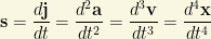
Jounce (also known as snap) is the fourth derivative of the position vector with respect to time, with the first, second, and third derivatives being velocity, acceleration, and jerk, respectively; in other words, jounce is the rate of change of the jerk with respect to time.
Physical dimensions of snap are
![\left[\mathbf{s}\right]=LT^{-4}](https://s0.wp.com/latex.php?latex=%5Cleft%5B%5Cmathbf%7Bs%7D%5Cright%5D%3DLT%5E%7B-4%7D&bg=f9f7e1&fg=000000&s=0&c=20201002)
5th and beyond: Higher-order derivatives
Following jounce (snap), the fifth and sixth derivatives of the displacement vector are sometimes referred to as crackle and pop, respectively. Dork has also been suggested for the sixth derivative. Although the reasons given were less than entirely sincere, dork does have an appealing ring to it, specially for geeks, freaks and dorks. The seventh and eighth derivatives of the displacement vector are sometimes referred to as lock and drop. Their respective formulae can be obtained in a simple way from the previous formalism.
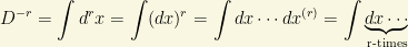
In general, physical dimensions of higher order derivatives of position are defined to be quantities with ![\left[\mathbf{Q}\right]=LT^{-r}](https://s0.wp.com/latex.php?latex=%5Cleft%5B%5Cmathbf%7BQ%7D%5Cright%5D%3DLT%5E%7B-r%7D&bg=f9f7e1&fg=000000&s=0&c=20201002)

-1st derivative (integral) of position is absement
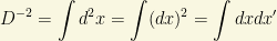
Absement (or absition) refers to the -1th time-derivative of displacement (or position), i.e. the integral of position over time. Mathematically speaking:

The rate of change of absement is position. Absement is a quantity with dimension 

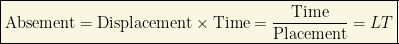
One meter-second corresponds to being absent from an origin or other reference point 1 meter away for a duration of one second. This amount of absement is equal to being two metres away from the origin for one half second, or being one half a metre from the origin for two seconds, or a 1mm absence for 1000 seconds, a 1km absence for 1 millisecond, and so on.
The word “absement” is a blend of the words absence and displacement.
The physical dimensions of absement are ![\left[\mathbf{A}\right]=LT](https://s0.wp.com/latex.php?latex=%5Cleft%5B%5Cmathbf%7BA%7D%5Cright%5D%3DLT&bg=f9f7e1&fg=000000&s=0&c=20201002)
Useful applications of absement
Whereas most musical keyboard instruments, such as the piano, and many electronic keyboards, respond to velocity at which keys are struck, and some such as the tracker-organ, respond to displacement (how far down a key is pressed), flow-based musical instruments such as the hydraulophone, respond to the integral of displacement, i.e. to a time-distance product. Thus “pressing” a key (water jet) on a hydraulophone down for a longer period of time will result in a buildup of the sound level, as fluid (water) begins to fill the sounding mechanism (reservoir), up to a certain maximum filling point beyond which the sound levels off (along with a slow decay). Hydraulophone reservoirs have an approximate integrating effect on the distance or displacement applied by the musician’s fingers to the “keys” (water jets). Whereas the piano provides more articulation and enunciation of individual note-onsets than the organ, the hydraulophone provides a more continuously fluidly varying sound than either the organ or piano.
Of course all these models are approximate: hydraulophones are approximately presement-responsive, pianos are approximately velocity-responsive, etc..
The concepts of absement and presement originated in regards to flow-based musical instruments like hydraulophones, but may be applied to any area of physics, as they exist along the hierarchy of the derivatives of displacement.
A very slow-responding pipe-organ with tracker-action can often exhibit an effect similar to that of a hydraulophone, when it takes time for the wind and sound levels to build up, so that the sound level is approximately the product of how far down a key is pressed and how long it is held down for.
The concept of absement may also be applied to communications theory. For example, the difficulty in maintaining a communications channel (wired or wireless) increases with distance as well as with the time for which the channel must be kept active.
As a crude but simple example, absement may be used, very approximately, to model the cost of a long-distance phone call as the product of distance and time. A short-duration call over a long distance might, for example, represent the same quantity of absement as a long-duration call over a shorter distance.
Absement may also be used in sociological studies, i.e. we might express loneliness or homesickness as a product of distance from home and time away from home. Simply put, the old aphorism “absence makes the heart grow fonder” has been expressed as “absement makes the heart grow fonder”, to suggest that it matters both how absent one is (i.e. how far), as well as for how long one is absent.
Absement versus presement
Absement refers to the time-distance product (or more precisely the integral of displacement) away from a reference point, whereas the integral of reciprocal position, called presement, refers to the closeness, compounded over time.
The word “presement” is a portmanteau constructed from the words presence and displacement.
Placement (scalar quantity, nearness) is defined as the reciprocal of the position’s magnitude ( i.e., the reciprocal of the distance, an scalar quantity), and presement refers to the time-integral of placement. Most notably, with some high-pressure hydraulophones, it is physically impossible to fully obstruct a water jet, so position can never reach zero, and thus placement remains finite, as does its time integral, presement.
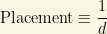

and where d is the distance 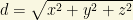
Physical dimensions of placement are ![\left[\mbox{Placement}\right]=L^{-1}](https://s0.wp.com/latex.php?latex=%5Cleft%5B%5Cmbox%7BPlacement%7D%5Cright%5D%3DL%5E%7B-1%7D&bg=f9f7e1&fg=000000&s=0&c=20201002)
![\left[\mbox{Presement}\right]=L^{-1}T](https://s0.wp.com/latex.php?latex=%5Cleft%5B%5Cmbox%7BPresement%7D%5Cright%5D%3DL%5E%7B-1%7DT&bg=f9f7e1&fg=000000&s=0&c=20201002)
Lower-order derivatives (higher-order integrals)
Some hydraulophones, such as the North Nessie (the hydraulophone on the North side of hydraulophone circle) at the Ontario Science Centre consist of cascaded hydraulophonic mechanisms, resulting in a double-integrating effect. In particular, the hydraulophone is linked indirectly to the North pipes, such that the water in direct physical contact with the fingers of the musician is not the same water in the organ pipes. As a result of this indirection, the instrument itself responds to presement/absement, the first integral of position whereas the pipes respond absemently to the action in the instrument, i.e. to the second integral of position of the player’s fingers. The time-integral of the time-integral of position is called absity/presity.
Absity is a portmanteau formed from the words absement (or absence) and velocity.
Following this pattern, higher time integrals of displacement may be named as follows:
1) Absement or absition is the integral of displacement.
2) Absity is the double integral of displacement.
3) Abseleration is the triple integral of displacement.
4) Abserk is the fourth integral of displacement.
5) Absounce is the fifth integral of displacement.
Likewise, presement, presity, preseleration, and similar words, are the integrals of reciprocal displacement (nearness).
Although there are no three-stage hydraulophones currently being manufactured as products, there are a number of three-stage (and some with higher numbers of stages) hydraulophone prototypes, in which some elements of the sound production respond to absity/presity, abseleration/preseleration, etc.
Derivatives of momentum
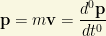
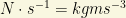
In Physics, momentum is defined as the product of mass and velocity, i.e.,

or mathematically speaking

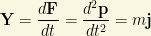
Moreover, we define the concept of “force” as the rate of change of momentum with respect to time, i.e.,

It mass does not depend on the time, we get

Can we define names for the next derivatives of momentum with respect to time? Of course, we can. It is only a nominal issue. There is a famous “poem” about this:
“Momentum equals mass times velocity. Force equals mass times acceleration. Yank equals mass times jerk. Tug equals mass times snap. Snatch equals mass times crackle. Shake equals mass times pop.”
If mass is not constant, the common definitions of higher derivatives of momentum are as follows ( the last equality is obtained supposing the mass is constant with time):
0th time derivative of momentum is of course The Momentum itself ( I am sorry, Mom-entum is not related with your Mom).
1st time derivative of momentum is The Force ( I am sorry. It is a Star Wars joke).

2nd time derivative of momentum is The Yank ( I am sorry, it is not a tank or a yankie from USA).
3rd time derivative of momentum is The Tug ( I am sorry. It is not a bug in the deepest part of The Matrix).

4th time derivative of momentum is The Snatch ( I am sorry, it is not the golden Snitch).

5th time derivative of momentum is The Shake ( I am sorry, it is not the japanese sake or a sweet tropical milk-shake).

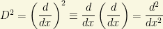
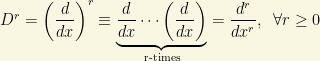
Notations for derivatives/integrals
Lebiniz operational notation: 


Newton dot notation: Derivatives are marked as dotted functions, e.g.,


Modern primed notation: Derivatives are marked as primed functions, e.g.,


Modern sublabel notation: Derivatives are marked with a subindex label denoting the variable with respect to we are making the derivative. Integrals are represented in the usual form. Thus,


These notations have their own advantanges and disadvantanges, but if we use them carefully, any of them can be very powerful.
Remarkable relationships
Physicists like to relate physical quantities in Mechanics/Dynamics to 4 main variables: force, power, action and energy. We can even dedude some interesting relationships between them and displacement, time, momentum, absement, placement, and presement.
1) Equations relating force and other magnitudes. Force dimensions are 


2) Equations relating power and other magnitudes. Power dimensions are 


3) Equations relating action and other magnitudes. Action dimensions are 


4) Equations relating energy and other magnitudes. Energy dimensions are 


In the same way, we can also deduce more fascinating identities:


since we easily get


and of course
Moreover, we also have


or

and the next interesting result as well:

or equivalently

Music, elements and Physics
The inspiring guide to the new names and variables was the theory of hydraulophones and music. In fact, there is a recent proposal to classify every musical instrument according to its physical origin instead of the classical element. It also makes sense to present the four states-of-matter in increasing order of energy: Earth/Solid first, Water/Liquid second, Air/Gas third, and Fire/Plasma fourth. At absolute zero, if it were possible, everything is a solid. then as things heat up they melt, then they evaporate, and finally, with enough energy, would become a ball of plasma, thus establishing a natural physical ordering as follows:
1) Earth/Solid played instruments. Geolophones. They produce sound pulsing the matter (“Earth”) of some object (string, membrane,…). Ordered in increasing dimension, from 1d to 3d, they can be: I) Chordophones (Played strings, streched objects with cross-section negligible respect to their length), II) Membranophones (Played membranes with thickness negligible respect to their area), III) Idiophones/Bulkphones (played 3d tensionless branes or higher).
2) Water/Liquid played instruments. Hydraulophones. These instruments produce vibrating sound pulsing jets of liquids (“Water”).
3) Air/Gas played instruments. Aerophones. These instuments produce vibrations and sound touching the flux of gases (“Air”).
4) Fire/Plasma played instruments. Ionophones. These instruments produce sonic waves playing the flux of plasma (“Fire”).
5) Quintessence/Idea/Information/Informatics played instruments. These instruments produce “sound” by computational means, whether optical, mechanical, electrical, or otherwise. We could name these instruments with some cool word. Akashaphones (from the sanskrit word/prefix “akasha”, meaning “aether, ether” or as Western tradition would say, “quintessence, fifth element”) will be the names of such instruments.
This classification matches the range of acoustic transducers that exist today (excepting the quintessencial transducer, of course) as well: 1) Geophone, 2) Hydrophone, 3) Microphone or speaker, and 4) Ionophone. In the same way I have never known a term for the akashaphones before, for the fifth transducer we should use a new term. Loakashaphone, from the same sanskrit origin than akashaphone, would be the analogue 5th transducer.
Summary
The following list is a summary of the derivatives of displacement/position:
A) Time integrals of position/displacement.
Order -9. Absrop. SI units 

Order -8. Absock. SI units 

Order -7. Absop. SI units 

Order -6. Absrackle. SI units 

Order -5. Absounce. SI units 

Order -4. Abserk. SI units 

Order -3. Abseleration. SI units 

Order -2. Absity. SI units 

Order -1. Absement. SI units
Order 0. Position/Displacement. SI units 

Remark: Integrals with respect to time of position measure “farness”.
B) Time derivatives of position/displacement.
Order 0. Position/Displacement. SI units
Order 1. Velocity. SI units 

Order 2. Acceleration. SI units
Order 3. Jerk/jolt/surge/lurch. SI units 

Order 4. Jounce/snap. SI units 

Order 5. Crackle. SI units 

Order 6. Pop. SI units 

Order 7. Lock. SI units 

Order 8. Drop. SI units 

Remark: Derivatives of position with respect to time measure “swiftness”.
C) Reciprocals of position/displacement and their time integrals.
Order 0. Placement. SI units 


Order -1. Presement. SI units 

Order -2. Presity. SI units 

Order -3. Preseleration. SI units 

Order -4. Preserk. SI units 

Order -5. Presounce. SI units 

Order -6. Presackle. SI units 

Order -7. Presop. SI units 

Order -8. Presock. SI units 

Order -9. Presrop. SI units 

Remark: Integrals of reciprocal displacement with respect to time measure “nearness”.
D) Time derivatives of momentum.
Order 0. Momentum. 


Order 1. Force. 

Order 2. Yank. 

Order 3. Tug. 

Order 4. Snatch. 

Order 5. Shake. 

Remark: Derivatives of momentum with respect to time measure “strengthness” or “forceness”.
So we have to remember 4 fascinating ideas,
i) Time integrals of position measure “farness”.
ii) Time derivatives of position measure “swiftness”.
iii) Time integrals of reciprocal position measure “nearness”.
iv) Time derivatives of momentum measure “forceness”.
And a fifth further great idea… Physics, Mathematics or more generally Physmatics own an inner “Harmony” or “Music” in their deepest principles and theories.
Some additional questions can be asked further:
0th. What about “infinite” order derivatives and integrals?
1st. What if time is not a continuous function?
2nd. What if time is not a scalar quantity?
3rd. What about fractional order/irrational order/complex order derivatives/X-order derivatives?
4th. What if (space) time/displacement does not exist?
5th. Can Mechanics/Dynamics of particles/fields/strings/branes/… be formulated in terms of integrals/reciprocals of “position” and “momentum” variables, i.e., as the power of negative and/or higher/lower derivatives? Would such a formulation of Mechanics/Dynamics be useful/meaningful for something deeper? That is, what are the right variables to study in Dynamics if some classical/quantum concepts are absent?
We could answer to some of these questions. For instance, the answer to the 0th question is interesting but it requires to know about jet spaces and/or path integrals. Moreover, the solution to the 3rd question would require the introduction of the fractional/fractal calculus. But that is another long story/log-entry to be told in a forthcoming future post!
Stay tuned!


You must be logged in to post a comment.